The hardware and bandwidth for this mirror is donated by dogado GmbH, the Webhosting and Full Service-Cloud Provider. Check out our Wordpress Tutorial.
If you wish to report a bug, or if you are interested in having us mirror your free-software or open-source project, please feel free to contact us at mirror[@]dogado.de.
Provide functionality for cancer subtyping using existing published methods or machine learning based on TCGA data.
Currently support mRNA subtyping:
1.0.0
You can install the released version through:
install.packages("OncoSubtype")This is a basic example for predicting the subtypes for Lung Squamous Cell Carcinoma (LUSC).
library(OncoSubtype)
library(tidyverse)
data <- get_median_centered(example_fpkm)
data <- assays(data)$centered
rownames(data) <- rowData(example_fpkm)$external_gene_name
# use default wilkerson's method
output1 <- centroids_subtype(data, disease = 'LUSC')
table(output1@subtypes)
#>
#>     basal classical primitive secretory
#> 44 65 26 44output2 <- ml_subtype(data, disease = 'LUSC', method = 'rf', seed = 123)
table(output2@subtypes)
#>
#> basal classical primitive secretory
#> 43 65 27 44confusionMatrix(as.factor(tolower(output1@subtypes)),
as.factor(tolower(output2@subtypes)))
#> Confusion Matrix and Statistics
#>
#> Reference
#> Prediction basal classical primitive secretory
#> basal 43 1 0 0
#> classical 0 64 1 0
#> primitive 0 0 26 0
#> secretory 0 0 0 44
#>
#> Overall Statistics
#>
#> Accuracy : 0.9888
#> 95% CI : (0.9602, 0.9986)
#> No Information Rate : 0.3631
#> P-Value [Acc > NIR] : < 2.2e-16
#>
#> Kappa : 0.9846
#>
#> Mcnemar's Test P-Value : NA
#>
#> Statistics by Class:
#>
#> Class: basal Class: classical Class: primitive
#> Sensitivity 1.0000 0.9846 0.9630
#> Specificity 0.9926 0.9912 1.0000
#> Pos Pred Value 0.9773 0.9846 1.0000
#> Neg Pred Value 1.0000 0.9912 0.9935
#> Prevalence 0.2402 0.3631 0.1508
#> Detection Rate 0.2402 0.3575 0.1453
#> Detection Prevalence 0.2458 0.3631 0.1453
#> Balanced Accuracy 0.9963 0.9879 0.9815
#> Class: secretory
#> Sensitivity 1.0000
#> Specificity 1.0000
#> Pos Pred Value 1.0000
#> Neg Pred Value 1.0000
#> Prevalence 0.2458
#> Detection Rate 0.2458
#> Detection Prevalence 0.2458
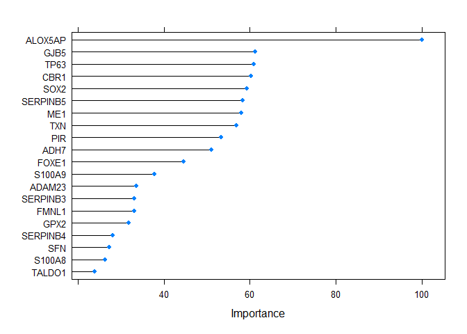
#> Balanced Accuracy 1.0000vi <- varImp(output2@method, scale = TRUE)
plot(vi, top = 20)
PlotHeat(object = output2, set = 'both', fontsize = 10,
        show_rownames = FALSE, show_colnames = FALSE)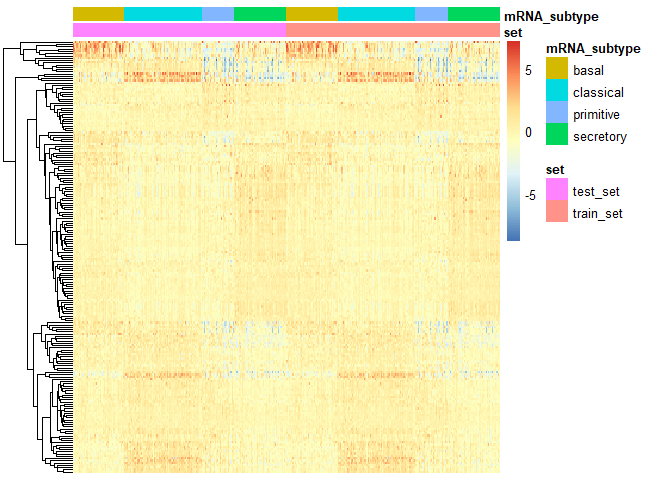
These binaries (installable software) and packages are in development.
They may not be fully stable and should be used with caution. We make no claims about them.
Health stats visible at Monitor.