The hardware and bandwidth for this mirror is donated by dogado GmbH, the Webhosting and Full Service-Cloud Provider. Check out our Wordpress Tutorial.
If you wish to report a bug, or if you are interested in having us mirror your free-software or open-source project, please feel free to contact us at mirror[@]dogado.de.

OTBsegm

OTBsegm is an R package that provides a user-friendly interface to the unsupervised image segmentation algorithms available in Orfeo ToolBox (OTB), a powerful open-source library for remote sensing image processing. OTBsegm is built on top of link2GI R package, providing easy access to image segmentation algorithms.

To use {OTBsegm}, you must first install OTB on your machine. Once OTB is installed and properly linked through {link2GI} (see examples), this package allows you to easily integrate OTB’s segmentation algorithms into your workflows.

Installation

You can install the development version of OTBsegm from GitHub with:

# install.packages("pak")
pak::pak("Cidree/OTBsegm")

Example

We will see how to segment an image included in the package:

## load packages
library(link2GI)
library(OTBsegm)
library(terra)
#> Warning: package 'terra' was built under R version 4.4.3
#> terra 1.8.29

## load image
image_sr <- rast(system.file("raster/pnoa.tiff", package = "OTBsegm"))

## visualize
plotRGB(image_sr)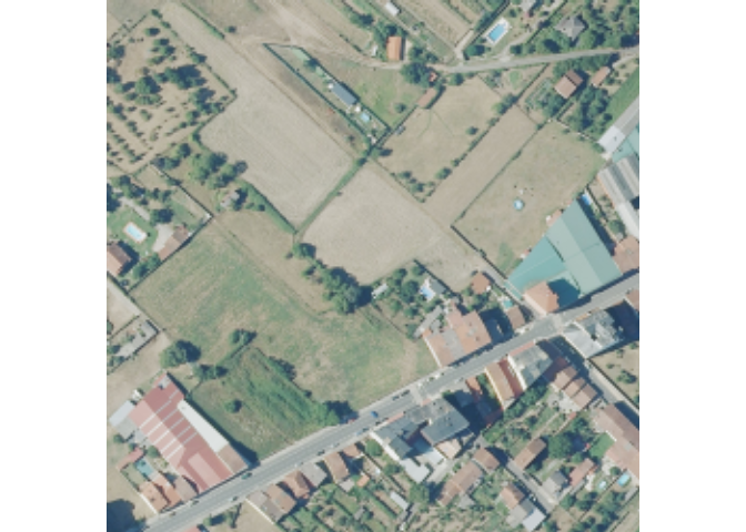

The image is a 500x500 meters RGB tile, with a spatial resolution of 15 cm in Galicia, Spain. The meanshift algorithm has the next important arguments:

• spatialr: spatial radius of the neighborhood

• ranger: range radius defining the radius (expressed in radiometry unit) in the multispectral space

• minsize: minimum size of a region (in pixel unit) in segmentation. Smaller clusters will be merged to the neighboring cluster with the closest radiometry. If set to 0 no pruning is done. The image’s resolution is 1.2 m, therefore, a value of minsize = 10 means that the smallest segment will be \(10 * 1.2^2 = 14.4 m^2\).

In order to use the algorithms, we need to link our OTB installation using {link2GI}:

otblink <- link2GI::linkOTB(searchLocation = "C:/OTB/")

Once we are connected, we can apply the segmentation algorithm and visualize the results:

results_ms_sf <- segm_meanshift(
    image    = image_sr,
    otb      = otblink,
    spatialr = 5,
    ranger   = 25,
    maxiter  = 10,
    minsize  = 10
)
#> Reading layer `filecfc6b37181f' from data source 
#>   `C:\Users\User\AppData\Local\Temp\RtmpAjZLFx\filecfc6b37181f.shp' 
#>   using driver `ESRI Shapefile'
#> Simple feature collection with 811 features and 1 field
#> Geometry type: POLYGON
#> Dimension:     XY
#> Bounding box:  xmin: 621000 ymin: 4708385 xmax: 621300 ymax: 4708685
#> Projected CRS: ETRS89 / UTM zone 29N

plotRGB(image_sr)
plot(sf::st_geometry(results_ms_sf), add = TRUE)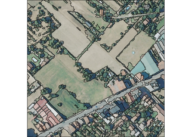

These binaries (installable software) and packages are in development.
They may not be fully stable and should be used with caution. We make no claims about them.
Health stats visible at Monitor.