The hardware and bandwidth for this mirror is donated by dogado GmbH, the Webhosting and Full Service-Cloud Provider. Check out our Wordpress Tutorial.
If you wish to report a bug, or if you are interested in having us mirror your free-software or open-source project, please feel free to contact us at mirror[@]dogado.de.
![]()
![]()
performs Bayesian wavelet analysis using individual non-local priors as described in Sanyal & Ferreira (2017) and non-local prior mixtures as described in Sanyal (2025).
You can install the development version of NLPwavelet like so:
install.packages("NLPwavelet")# install.packages("devtools")
devtools::install_github("nilotpalsanyal/NLPwavelet")BNLPWA is the main function of this package that performs Bayesian wavelet analysis using individual non-local priors as described in Sanyal & Ferreira (2017) and non-local prior mixtures as described in Sanyal (2025). It currently works with one-dimensional data. The usage is described below.
library(NLPwavelet)
#>
#>  Welcome to NLPwavelet!
#>
#>  Website: https://nilotpalsanyal.github.io/NLPwavelet/
#>  Bug report: https://github.com/nilotpalsanyal/NLPwavelet/issues

# Using the well-known Doppler function to
# illustrate the use of the function BNLPWA

# set seed for reproducibility
set.seed(1)

# Define the doppler function
doppler <- function(x) {
  sqrt(x * (1 - x)) * sin((2 * pi * 1.05) / (x + 0.05))
}

# Generate true values over a grid
n <- 512  # Number of points
x <- seq(0, 1, length.out = n)
true_signal <- doppler(x)

# Add noise to generate data
sigma <- 0.2  # Noise level
y <- true_signal + rnorm(n, mean = 0, sd = sigma)

# BNLPWA analysis based on MOM prior using logit specification
# for the mixture probabilities and polynomial decay
# specification for the scale parameter
fit_mom <- BNLPWA(data=y, func=true_signal, r=1, wave.family=
  "DaubLeAsymm", filter.number=6, bc="periodic", method="mom",
  mixprob_dist="logit", scale_dist="polynom")

plot(y,type="l",col="grey") # plot of data
lines(fit_mom$func.post.mean,col="blue") # plot of posterior 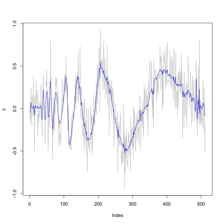
# smoothed estimates
fit_mom$MSE.mean
#> [1] 0.006592428

# BNLPWA analysis using non-local prior mixtures using generalized
# logit (Richard's) specification for the mixture probabilities and
# double exponential decay specification for the scale parameter
fit_mixture <- BNLPWA(data=y, func=true_signal, r=1, nu=1, wave.family=
  "DaubLeAsymm", filter.number=6, bc="periodic", method="mixture",
  mixprob_dist="genlogit", scale_dist="doubleexp")

plot(y,type="l",col="grey") # plot of data
lines(fit_mixture$func.post.mean,col="blue") # plot of posterior 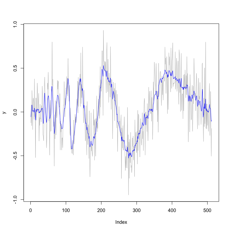
# smoothed estimates
fit_mixture$MSE.mean
#> [1] 0.006335836

# Compare with other wavelet methods
library(wavethresh)
#> Loading required package: MASS
#> WaveThresh: R wavelet software, release 4.7.2, installed
#> Copyright Guy Nason and others 1993-2022
#> Note: nlevels has been renamed to nlevelsWT
wd <- wd(y, family="DaubLeAsymm", filter.number=6, bc="periodic")  # Wavelet decomposition

wd_thresh_universal <- threshold(wd, policy="universal", type="hard")
fit_universal <- wr(wd_thresh_universal)
MSE_universal <- mean((true_signal-fit_universal)^2)
MSE_universal
#> [1] 0.009054956

wd_thresh_sure <- threshold(wd, policy="sure", type="soft")
fit_sure <- wr(wd_thresh_sure)
MSE_sure <- mean((true_signal-fit_sure)^2)
MSE_sure
#> [1] 0.01758871

wd_thresh_BayesThresh <- threshold(wd, policy="BayesThresh", type="hard")
fit_BayesThresh <- wr(wd_thresh_BayesThresh)
MSE_BayesThresh <- mean((true_signal-fit_BayesThresh)^2)
MSE_BayesThresh
#> [1] 0.007527764

wd_thresh_cv <- threshold(wd, policy="cv", type="hard")
fit_cv <- wr(wd_thresh_cv)
MSE_cv <- mean((true_signal-fit_cv)^2)
MSE_cv
#> [1] 0.008710683

wd_thresh_fdr <- threshold(wd, policy="fdr", type="hard")
fit_fdr <- wr(wd_thresh_fdr)
MSE_fdr <- mean((true_signal-fit_fdr)^2)
MSE_fdr
#> [1] 0.007777847

# Compare with non-wavelet methods
    # Kernel smoothing
fit_ksmooth <- ksmooth(x, y, kernel="normal", bandwidth=0.05)
MSE_ksmooth <- mean((true_signal-fit_ksmooth$y)^2)
MSE_ksmooth
#> [1] 0.01518292
    # LOESS smoothing
fit_loess <- loess(y ~ x, span=0.1)  # Adjust span for more or less smoothing
MSE_loess <- mean((true_signal-predict(fit_loess))^2)
MSE_loess
#> [1] 0.01059615
    # Cubic spline smoothing
spline_fit <- smooth.spline(x, y, spar=0.5)  # Adjust spar for smoothness
MSE_spline <- mean((true_signal-spline_fit$y)^2)
MSE_spline
#> [1] 0.01083473Sanyal, Nilotpal, and Marco AR Ferreira. “Bayesian wavelet analysis using nonlocal priors with an application to FMRI analysis.” Sankhya B 79.2 (2017): 361-388. https://doi.org/10.1007/s13571-016-0129-3
Sanyal, Nilotpal. “Nonlocal prior mixture-based Bayesian wavelet regression.” arXiv preprint arXiv:2501.18134 (2025). https://doi.org/10.48550/arXiv.2501.18134
These binaries (installable software) and packages are in development.
They may not be fully stable and should be used with caution. We make no claims about them.
Health stats visible at Monitor.