The hardware and bandwidth for this mirror is donated by dogado GmbH, the Webhosting and Full Service-Cloud Provider. Check out our Wordpress Tutorial.
If you wish to report a bug, or if you are interested in having us mirror your free-software or open-source project, please feel free to contact us at mirror[@]dogado.de.
![]()
A package that enables quantifying landscape diversity and structure at multiple scales. For these purposes Juhász-Nagy’s functions, i.e. compositional diversity (CD) and associatum (AS), are calculated.
You can install the development version of LandComp
using the following command:
install.packages("devtools")
devtools::install_github("ladylavender/LandComp")
Example regular grids represent demonstrative spatial arrangements.
They reflect a typical case when having presence/absence data on some
landscape classes (e.g. vegetation types here) along a landscape. Note,
there are three requirements of using the LandComp
package:
The structure and the visualization of the example square grid data:
suppressPackageStartupMessages(library("sf"))
library(LandComp)
data("square_data")
plot(square_data)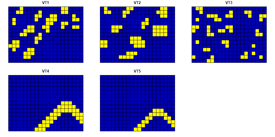
str(square_data)
#> Classes 'sf' and 'data.frame':   300 obs. of  6 variables:
#>  $ VT1     : num  0 0 0 0 0 0 0 0 0 0 ...
#>  $ VT2     : num  0 0 0 0 0 0 0 0 0 0 ...
#>  $ VT3     : num  0 0 0 0 1 1 0 0 0 0 ...
#>  $ VT4     : num  0 0 0 0 0 0 0 1 1 1 ...
#>  $ VT5     : num  0 0 0 0 0 0 0 0 0 1 ...
#>  $ geometry:sfc_POLYGON of length 300; first list element: List of 1
#>   ..$ : num [1:5, 1:2] 400000 400000 405000 405000 400000 ...
#>   ..- attr(*, "class")= chr [1:3] "XY" "POLYGON" "sfg"
#>  - attr(*, "sf_column")= chr "geometry"
#>  - attr(*, "agr")= Factor w/ 3 levels "constant","aggregate",..: NA NA NA NA NA
#>   ..- attr(*, "names")= chr [1:5] "VT1" "VT2" "VT3" "VT4" ...
Two values of CD and AS measuring landscape diversity and structure can be calculated as e.g.
LandComp(x = square_data, aggregation_steps = 0:1)
#>   AggregationStep SpatialUnit_Size SpatialUnit_Area SpatialUnit_Count
#> 1               0                1         2.50e+07               300
#> 2               1                9         2.25e+08               234
#>   UniqueCombination_Count   CD_bit    AS_bit
#> 1                      13 2.755349 0.1709469
#> 2 18 3.176364 1.0874836The structure and the visualization of the example hexagonal grid data:
data("hexagonal_data")
plot(hexagonal_data)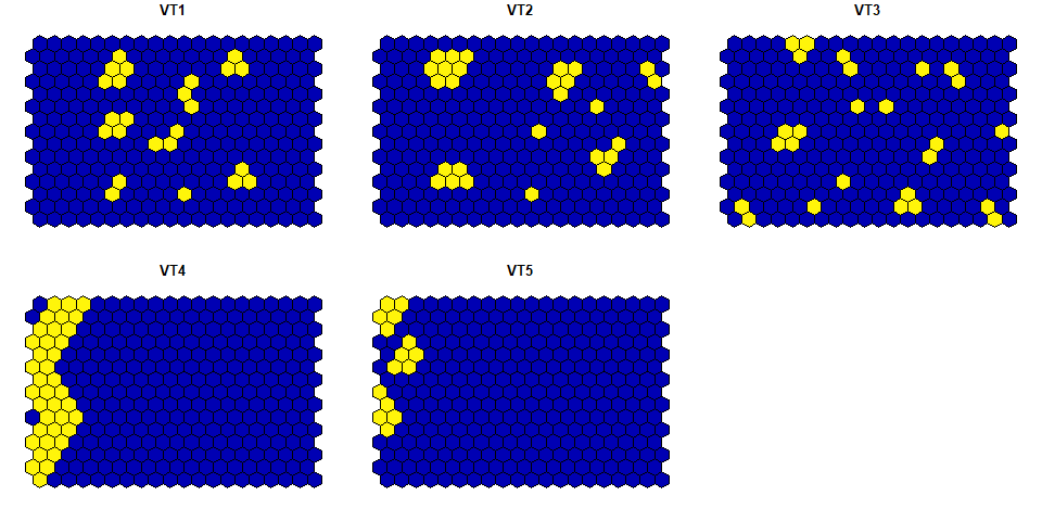
str(hexagonal_data)
#> Classes 'sf' and 'data.frame':   300 obs. of  6 variables:
#>  $ VT1     : num  0 0 0 0 0 0 0 0 0 0 ...
#>  $ VT2     : num  0 0 0 0 0 0 0 0 0 0 ...
#>  $ VT3     : num  0 0 0 0 0 0 0 0 0 0 ...
#>  $ VT4     : num  1 1 0 1 1 1 0 1 1 1 ...
#>  $ VT5     : num  0 0 1 1 0 0 1 0 0 1 ...
#>  $ geometry:sfc_POLYGON of length 300; first list element: List of 1
#>   ..$ : num [1:7, 1:2] 649500 649000 649000 649500 650000 ...
#>   ..- attr(*, "class")= chr [1:3] "XY" "POLYGON" "sfg"
#>  - attr(*, "sf_column")= chr "geometry"
#>  - attr(*, "agr")= Factor w/ 3 levels "constant","aggregate",..: NA NA NA NA NA
#> ..- attr(*, "names")= chr [1:5] "VT1" "VT2" "VT3" "VT4" ...LandComp(x = hexagonal_data, aggregation_steps = 0:1)
#> AggregationStep SpatialUnit_Size SpatialUnit_Area SpatialUnit_Count
#> 1 0 1 866025.4 300
#> 2 1 7 6062177.8 234
#> UniqueCombination_Count CD_bit AS_bit
#> 1 12 1.972863 0.1256525
#> 2 16 3.422409 0.5394512For further information and examples, see both the vignette of the
package and ?LandComp after installing the package.
Note, if you would like to view the vignette from R using the code
vignette("LandComp"), you should install the package using
the following command:
devtools::install_github("ladylavender/LandComp", build_vignettes = TRUE)These binaries (installable software) and packages are in development.
They may not be fully stable and should be used with caution. We make no claims about them.
Health stats visible at Monitor.