The hardware and bandwidth for this mirror is donated by dogado GmbH, the Webhosting and Full Service-Cloud Provider. Check out our Wordpress Tutorial.
If you wish to report a bug, or if you are interested in having us mirror your free-software or open-source project, please feel free to contact us at mirror[@]dogado.de.
Please feel free to create an issue for bug reports or potential improvements.
![]()
![]()
IRTest is a useful tool for \(\mathcal{\color{red}{IRT}}\) (item response theory) parameter \(\mathcal{\color{red}{est}}\textrm{imation}\), especially when the violation of normality assumption on latent distribution is suspected.
IRTest deals with uni-dimensional latent variable.
For missing values, IRTest adopts full information maximum likelihood (FIML) approach.
In IRTest, including the conventional usage of Gaussian distribution, several methods are available for estimation of latent distribution:
The CRAN version of IRTest can be installed on R-console with:
install.packages("IRTest")For the development version, it can be installed on R-console with:
devtools::install_github("SeewooLi/IRTest")Followings are the functions of IRTest.
IRTest_Dich is the estimation function when items
are dichotomously scored.
IRTest_Poly is the estimation function when items
are polytomously scored.
IRTest_Cont is the estimation function when items
are continuously scored.
IRTest_Mix is the estimation function for a
mixed-format test, a test comprising both dichotomous item(s) and
polytomous item(s).
factor_score estimates factor scores of
examinees.
coef_se returns standard errors of item parameter
estimates.
best_model selects the best model using an
evaluation criterion.
item_fit tests the statistical fit of all items
individually.
inform_f_item calculates the information value(s) of
an item.
inform_f_test calculates the information value(s) of
a test.
plot_item draws item response function(s) of an
item.
reliability calculates marginal reliability
coefficient of IRT.
latent_distribution returns evaluated PDF value(s)
of an estimated latent distribution.
DataGeneration generates several objects that can be
useful for computer simulation studies. Among these are simulated item
parameters, ability parameters and the corresponding item-response
data.
dist2 is a probability density function of
two-component Gaussian mixture distribution.
original_par_2GM converts re-parameterized
parameters of two-component Gaussian mixture distribution into original
parameters.
cat_clps recommends category collapsing based on
item parameters (or, equivalently, item response functions).
recategorize implements the category
collapsing.
For S3 methods, anova, coef,
logLik, plot, print, and
summary are available.
A simple simulation study for a 2PL model can be done in following manners:
library(IRTest)An artificial data of 1000 examinees and 20 items.
Alldata <- DataGeneration(seed = 123456789,
                          model_D = 2,
                          N=1000,
                          nitem_D = 10,
                          latent_dist = "2NM",
                          m=0, # mean of the latent distribution
                          s=1, # s.d. of the latent distribution
                          d = 1.664,
                          sd_ratio = 2,
                          prob = 0.3)

data <- Alldata$data_D
item <- Alldata$item_D
theta <- Alldata$theta
colnames(data) <- paste0("item",1:10)For an illustrative purpose, the two-component Gaussian mixture distribution (2NM) method is used for the estimation of latent distribution.
Mod1 <-
  IRTest_Dich(
    data = data,
    latent_dist = "2NM"
)summary(Mod1)
#> Convergence:
#> Successfully converged below the threshold of 1e-04 on 52nd iterations.
#>
#> Model Fit:
#> log-likeli -4786.735
#> deviance 9573.47
#> AIC 9619.47
#> BIC 9732.348
#> HQ 9662.371
#>
#> The Number of Parameters:
#> item 20
#> dist 3
#> total 23
#>
#> The Number of Items: 10
#>
#> The Estimated Latent Distribution:
#> method - 2NM
#> ----------------------------------------
#>
#>
#>
#> . @ @ .
#> . . @ @ @ @ .
#> @ @ @ . . . @ @ @ @ @ @
#> @ @ @ @ @ @ @ @ @ @ @ @ @ @
#> . @ @ @ @ @ @ @ @ @ @ @ @ @ @ @
#> @ @ @ @ @ @ @ @ @ @ @ @ @ @ @ @ .
#> @ @ @ @ @ @ @ @ @ @ @ @ @ @ @ @ @ @ @
#> +---------+---------+---------+---------+
#> -2 -1 0 1 2colnames(item) <- c("a", "b", "c")
knitr::kables(
list(
### True item parameters
knitr::kable(item, format='simple', caption = "True item parameters", digits = 2)%>%
kableExtra::kable_styling(font_size = 4),
### Estimated item parameters
knitr::kable(coef(Mod1), format='simple', caption = "Estimated item parameters", digits = 2)%>%
kableExtra::kable_styling(font_size = 4)
)
)
True item parameters |
Estimated item parameters |
### Plotting
fscores <- factor_score(Mod1, ability_method = "WLE")

par(mfrow=c(1,3))
plot(item[,1], Mod1$par_est[,1], xlab = "true", ylab = "estimated", main = "item discrimination parameters")
abline(a=0,b=1)
plot(item[,2], Mod1$par_est[,2], xlab = "true", ylab = "estimated", main = "item difficulty parameters")
abline(a=0,b=1)
plot(theta, fscores$theta, xlab = "true", ylab = "estimated", main = "ability parameters")
abline(a=0,b=1)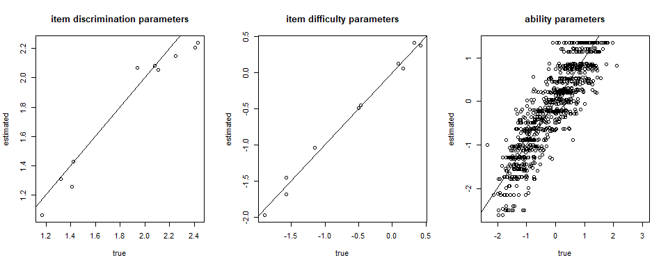
plot(Mod1, mapping = aes(colour="Estimated"), linewidth = 1) +
  stat_function(
    fun = dist2,
    args = list(prob = .3, d = 1.664, sd_ratio = 2),
    mapping = aes(colour = "True"),
    linewidth = 1) +
  lims(y = c(0, .75)) +
  labs(title="The estimated latent density using '2NM'", colour= "Type")+
  theme_bw()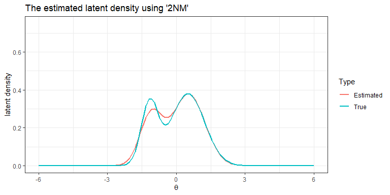
Each examinee’s posterior distribution is calculated in the E-step of
EM algorithm. Posterior distributions can be found in
Mod1$Pk.
set.seed(1)
selected_examinees <- sample(1:1000,6)
post_sample <-
  data.frame(
    X = rep(seq(-6,6, length.out=121),6),
    prior = rep(Mod1$Ak/(Mod1$quad[2]-Mod1$quad[1]), 6),
    posterior = 10*c(t(Mod1$Pk[selected_examinees,])),
    ID = rep(paste("examinee", selected_examinees), each=121)
    )

ggplot(data=post_sample, mapping=aes(x=X))+
  geom_line(mapping=aes(y=posterior, group=ID, color='Posterior'))+
  geom_line(mapping=aes(y=prior, group=ID, color='Prior'))+
  labs(title="Posterior densities for selected examinees", x=expression(theta), y='density')+
  facet_wrap(~ID, ncol=2)+
  theme_bw()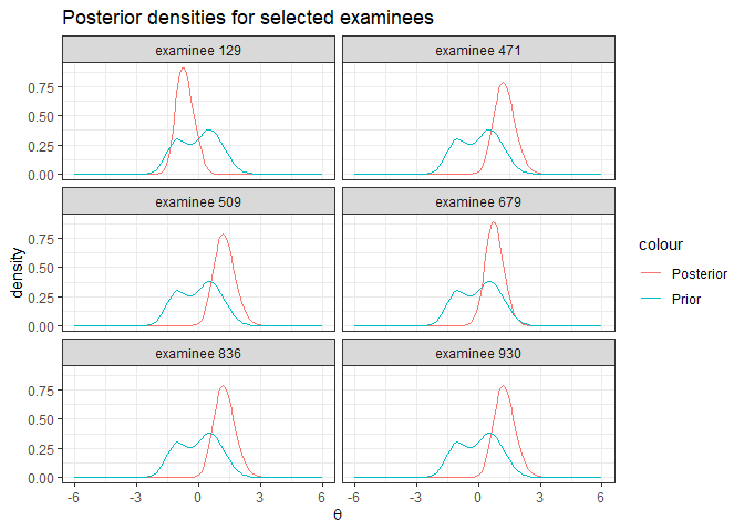
item_fit(Mod1)
#>            stat df p.value
#> item1  21.05671  5  0.0008
#> item2  39.02570  5  0.0000
#> item3  18.38362  5  0.0025
#> item4  26.05321  5  0.0001
#> item5  14.32944  5  0.0136
#> item6  38.58178  5  0.0000
#> item7  25.55813  5  0.0001
#> item8  14.43724  5  0.0131
#> item9  18.29168  5  0.0026
#> item10 65.25730 5 0.0000p1 <- plot_item(Mod1,1)
p2 <- plot_item(Mod1,4)
p3 <- plot_item(Mod1,8)
p4 <- plot_item(Mod1,10)
grid.arrange(p1, p2, p3, p4, ncol=2, nrow=2)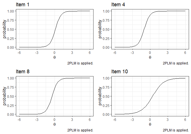
reliability(Mod1)
#> $summed.score.scale
#> $summed.score.scale$test
#> test reliability
#>        0.8133724
#>
#> $summed.score.scale$item
#>     item1     item2     item3     item4     item5     item6     item7     item8
#> 0.4586845 0.3014150 0.3020569 0.3805658 0.1425997 0.4534584 0.2689003 0.4475401
#>     item9    item10
#> 0.2661777 0.1963059
#>
#>
#> $theta.scale
#> test reliability
#> 0.7457059ggplot()+
stat_function(
fun = inform_f_test,
args = list(Mod1)
)+
stat_function(
fun=inform_f_item,
args = list(Mod1, 1),
mapping = aes(color="Item 1")
)+
stat_function(
fun=inform_f_item,
args = list(Mod1, 2),
mapping = aes(color="Item 2")
)+
stat_function(
fun=inform_f_item,
args = list(Mod1, 3),
mapping = aes(color="Item 3")
)+
stat_function(
fun=inform_f_item,
args = list(Mod1, 4),
mapping = aes(color="Item 4")
)+
stat_function(
fun=inform_f_item,
args = list(Mod1, 5),
mapping = aes(color="Item 5")
)+
lims(x=c(-6,6))+
labs(title="Test information function", x=expression(theta), y='information')+
theme_bw()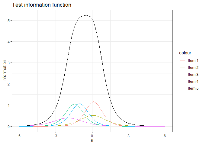
These binaries (installable software) and packages are in development.
They may not be fully stable and should be used with caution. We make no claims about them.
Health stats visible at Monitor.