The hardware and bandwidth for this mirror is donated by dogado GmbH, the Webhosting and Full Service-Cloud Provider. Check out our Wordpress Tutorial.
If you wish to report a bug, or if you are interested in having us mirror your free-software or open-source project, please feel free to contact us at mirror[@]dogado.de.
![]()
The goal of ICSClust is to perform tandem clustering
with invariant coordinate selection.
You can install the development version of ICSClust from GitHub with:
# install.packages("devtools")
devtools::install_github("AuroreAA/ICSClust")library(ICSClust)
#> Loading required package: ICS
#> Loading required package: mvtnorm
#> Loading required package: ggplot2
#> Registered S3 method overwritten by 'GGally':
#> method from
#> +.gg ggplot2
# import data
X <- iris[,-5]
# run ICS
ICS_out <- ICS(X)
summary(ICS_out)
#>
#> ICS based on two scatter matrices
#> S1: COV
#> S2: COV4
#>
#> Information on the algorithm:
#> QR: TRUE
#> whiten: FALSE
#> center: FALSE
#> fix_signs: scores
#>
#> The generalized kurtosis measures of the components are:
#> IC.1 IC.2 IC.3 IC.4
#> 1.2074 1.0269 0.9292 0.7405
#>
#> The coefficient matrix of the linear transformation is:
#> Sepal.Length Sepal.Width Petal.Length Petal.Width
#> IC.1 -0.52335 1.9933 2.3731 -4.4308
#> IC.2 0.83296 1.3275 -1.2666 2.7900
#> IC.3 3.05683 -2.2269 -1.6354 0.3654
#> IC.4 0.05244 0.6032 -0.3483 -0.3798
# Pot of generalized eigenvalues
select_plot(ICS_out)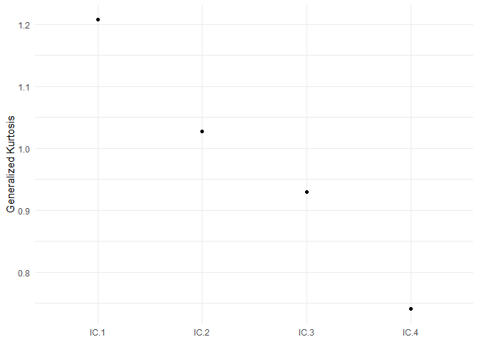
select_plot(ICS_out, type = "lines")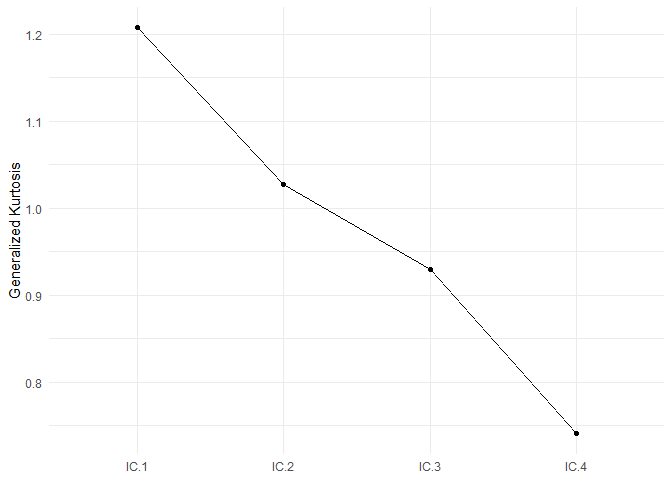
# pairs of all components
component_plot(ICS_out)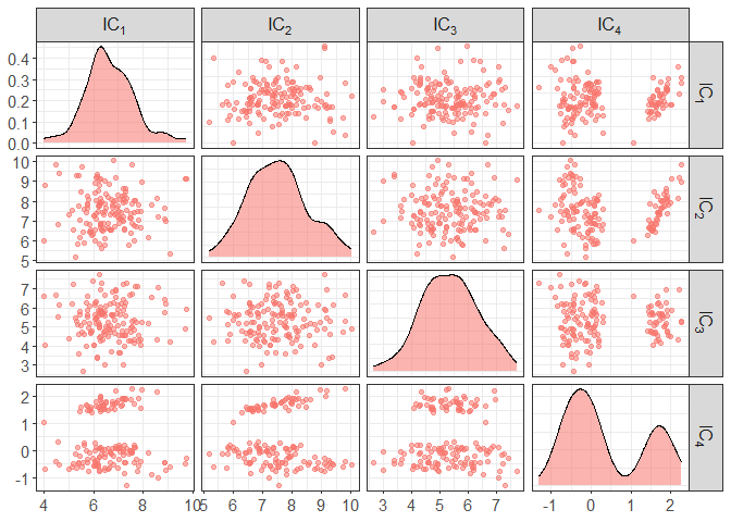
# pairs of only a the first and fourth components
component_plot(ICS_out, select = c(1,4))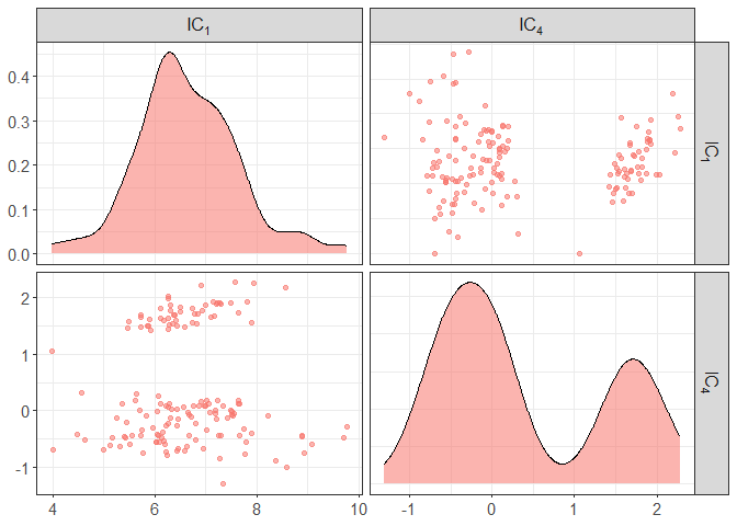
# add some colors by clusters
component_plot(ICS_out, clusters = iris[,5])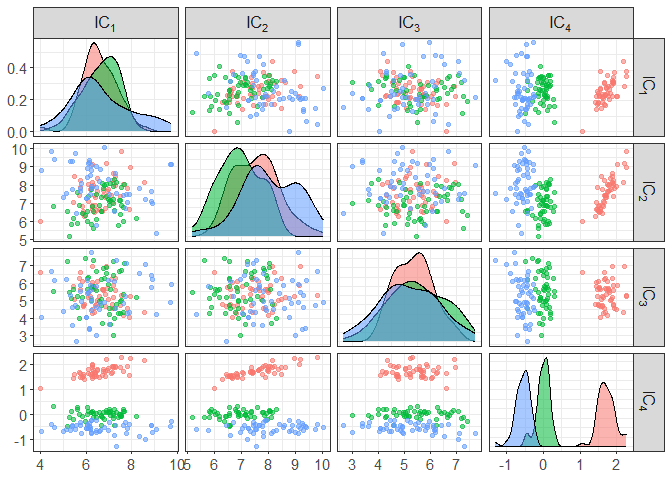
component_plot(ICS_out, select = c(1,4), clusters = iris[,5])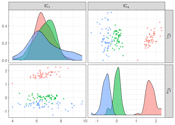
# in case you want to do it for initial data
component_plot(X, select = c(1,4), clusters = iris[,5])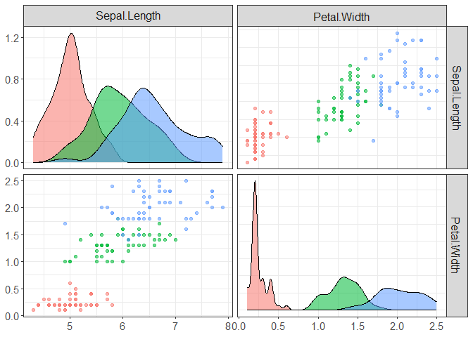
# ICSClust requires at least 2 arguments:
# - X: data
# - nb_clusters: nb of clusters
ICS_out <- ICSClust(X, nb_clusters = 3)
summary(ICS_out)
#>
#> ICS based on two scatter matrices
#> S1: COV
#> S2: COV4
#>
#> The generalized kurtosis measures of the components are:
#>   IC.1   IC.2   IC.3   IC.4
#> 1.2074 1.0269 0.9292 0.7405
#>
#> The coefficient matrix of the linear transformation is:
#>      Sepal.Length Sepal.Width Petal.Length Petal.Width
#> IC.1     -0.52335      1.9933       2.3731     -4.4308
#> IC.2      0.83296      1.3275      -1.2666      2.7900
#> IC.3      3.05683     -2.2269      -1.6354      0.3654
#> IC.4      0.05244      0.6032      -0.3483     -0.3798
#>
#>  3 components are selected: IC.4 IC.1 IC.2
#>
#>  3 clusters are identified:
#>
#>  1  2  3
#> 38 62 50
plot(ICS_out)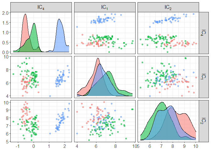
# You can also mention the number of invariant components to keep
ICS_out <- ICSClust(X, nb_select = 2, nb_clusters = 3)
# confusion table with initial clusters
table(ICS_out$clusters, iris[,5])
#>
#>     setosa versicolor virginica
#>   1      0         25        19
#>   2     49          0         0
#>   3      1         25        31
component_plot(ICS_out$ICS_out, select = ICS_out$select, clusters = as.factor(ICS_out$clusters))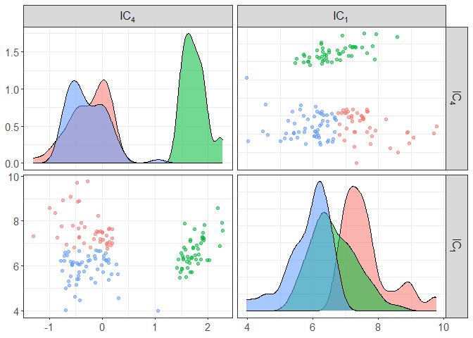
# to change the scatter pair
ICS_out <- ICSClust(X, nb_select = 1, nb_clusters = 3,
                ICS_args = list(S1 = ICS_mcd_raw, S2 = ICS_cov,
                                S1_args = list(alpha = 0.5)))
table(ICS_out$clusters, iris[,5])
#>
#>     setosa versicolor virginica
#>   1      0          5        26
#>   2      0         45        24
#>   3     50          0         0
component_plot(ICS_out$ICS_out, clusters = as.factor(ICS_out$clusters))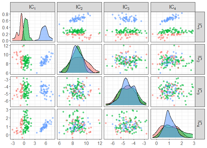
# to change the criteria to select the invariant components
ICS_out <- ICSClust(X, nb_clusters = 3,
                ICS_args = list(S1 = ICS_mcd_raw, S2 = ICS_cov,
                                S1_args = list(alpha = 0.5)),
                criterion = "normal_crit",
                ICS_crit_args = list(level = 0.1, test = "anscombe.test",
                                     max_select = NULL))

component_plot(ICS_out$ICS_out, select = ICS_out$select, clusters = as.factor(ICS_out$clusters))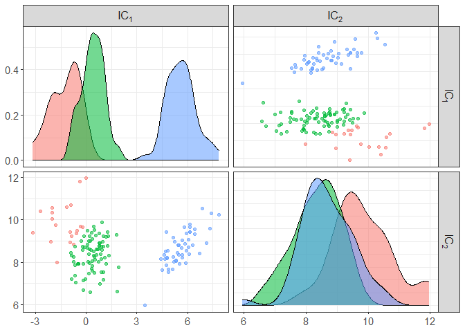
# to change the clustering method
ICS_out <- ICSClust(X, nb_select = 1, nb_clusters = 3,
                ICS_args = list(S1 = ICS_mcd_raw, S2 = ICS_cov,
                                S1_args = list(alpha = 0.5)),
                method  = "tkmeans_clust",
                clustering_args = list(alpha = 0.1))
table(ICS_out$clusters, iris[,5])
#>
#>     setosa versicolor virginica
#>   0      7          0         8
#>   1      0         40        15
#>   2     43          0         0
#>   3      0         10        27
component_plot(ICS_out$ICS_out, clusters = as.factor(ICS_out$clusters))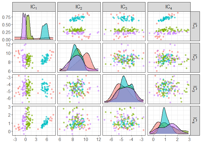
These binaries (installable software) and packages are in development.
They may not be fully stable and should be used with caution. We make no claims about them.
Health stats visible at Monitor.