The hardware and bandwidth for this mirror is donated by dogado GmbH, the Webhosting and Full Service-Cloud Provider. Check out our Wordpress Tutorial.
If you wish to report a bug, or if you are interested in having us mirror your free-software or open-source project, please feel free to contact us at mirror[@]dogado.de.

The R package FFTrees creates, visualizes and evaluates fast-and-frugal decision trees (FFTs) for solving binary classification tasks, using the algorithms and methods described in Phillips, Neth, Woike & Gaissmaier (2017, 10.1017/S1930297500006239).
Fast-and-frugal trees (FFTs) are simple and transparent decision algorithms for solving binary classification problems. The key feature making FFTs faster and more frugal than other decision trees is that every node allows making a decision. When predicting novel cases, the performance of FFTs competes with more complex algorithms and machine learning techniques, such as logistic regression (LR), support-vector machines (SVM), and random forests (RF). Apart from being faster and requiring less information, FFTs tend to be robust against overfitting, and are easy to interpret, use, and communicate.
The latest release of FFTrees is available from CRAN at https://CRAN.R-project.org/package=FFTrees:
install.packages("FFTrees")The current development version can be installed from its GitHub repository at https://github.com/ndphillips/FFTrees:
# install.packages("devtools")
devtools::install_github("ndphillips/FFTrees", build_vignettes = TRUE)As an example, let’s create a FFT predicting patients’ heart disease
status (Healthy vs. Disease) based on the
heartdisease dataset included in
FFTrees:
library(FFTrees) # load packageThe heartdisease data provides medical information for
303 patients that were examined for heart disease. The full data
contains a binary criterion variable describing the true state of each
patient and were split into two subsets: A heart.train set
for fitting decision trees, and heart.test set for a
testing these trees. Here are the first rows and columns of both subsets
of the heartdisease data:
heart.train (the training / fitting data) describes 150
patients:| diagnosis | age | sex | cp | trestbps | chol | fbs | restecg | thalach | exang | oldpeak | slope | ca | thal |
|---|---|---|---|---|---|---|---|---|---|---|---|---|---|
| FALSE | 44 | 0 | np | 108 | 141 | 0 | normal | 175 | 0 | 0.6 | flat | 0 | normal |
| FALSE | 51 | 0 | np | 140 | 308 | 0 | hypertrophy | 142 | 0 | 1.5 | up | 1 | normal |
| FALSE | 52 | 1 | np | 138 | 223 | 0 | normal | 169 | 0 | 0.0 | up | 1 | normal |
| TRUE | 48 | 1 | aa | 110 | 229 | 0 | normal | 168 | 0 | 1.0 | down | 0 | rd |
| FALSE | 59 | 1 | aa | 140 | 221 | 0 | normal | 164 | 1 | 0.0 | up | 0 | normal |
| FALSE | 58 | 1 | np | 105 | 240 | 0 | hypertrophy | 154 | 1 | 0.6 | flat | 0 | rd |
Table 1: Beginning of the heart.train
subset (using the data of 150 patients for fitting/training FFTs).
heart.test (the testing / prediction data) describes
153 different patients on the same variables:| diagnosis | age | sex | cp | trestbps | chol | fbs | restecg | thalach | exang | oldpeak | slope | ca | thal |
|---|---|---|---|---|---|---|---|---|---|---|---|---|---|
| FALSE | 51 | 0 | np | 120 | 295 | 0 | hypertrophy | 157 | 0 | 0.6 | up | 0 | normal |
| TRUE | 45 | 1 | ta | 110 | 264 | 0 | normal | 132 | 0 | 1.2 | flat | 0 | rd |
| TRUE | 53 | 1 | a | 123 | 282 | 0 | normal | 95 | 1 | 2.0 | flat | 2 | rd |
| TRUE | 45 | 1 | a | 142 | 309 | 0 | hypertrophy | 147 | 1 | 0.0 | flat | 3 | rd |
| FALSE | 66 | 1 | a | 120 | 302 | 0 | hypertrophy | 151 | 0 | 0.4 | flat | 0 | normal |
| TRUE | 48 | 1 | a | 130 | 256 | 1 | hypertrophy | 150 | 1 | 0.0 | up | 2 | rd |
Table 2: Beginning of the heart.test
subset (used to predict diagnosis for 153 new
patients).
Our challenge is to predict each patient’s diagnosis — a
column of logical values indicating the true state of each patient
(i.e., TRUE or FALSE, based on the patient
suffering or not suffering from heart disease) — from the values of
potential predictors.
To solve binary classification problems by FFTs, we must answer two key questions:
Once we have created some FFTs, additional questions include:
The FFTrees package answers these questions by creating, evaluating, and visualizing FFTs.
We use the main FFTrees() function to create FFTs for
the heart.train data and evaluate their predictive
performance on the heart.test data:
FFTrees() function allows creating an
FFTrees object for the heartdisease data:# Create an FFTrees object from the heartdisease data:
heart_fft <- FFTrees(formula = diagnosis ~.,
data = heart.train,
data.test = heart.test,
decision.labels = c("Healthy", "Disease"))Evaluating FFTrees() analyzes the training data, creates
several FFTs, and applies them to the test data. The results are stored
in an object heart_fft, which can be printed, plotted and
summarized (with options for selecting specific data or trees).
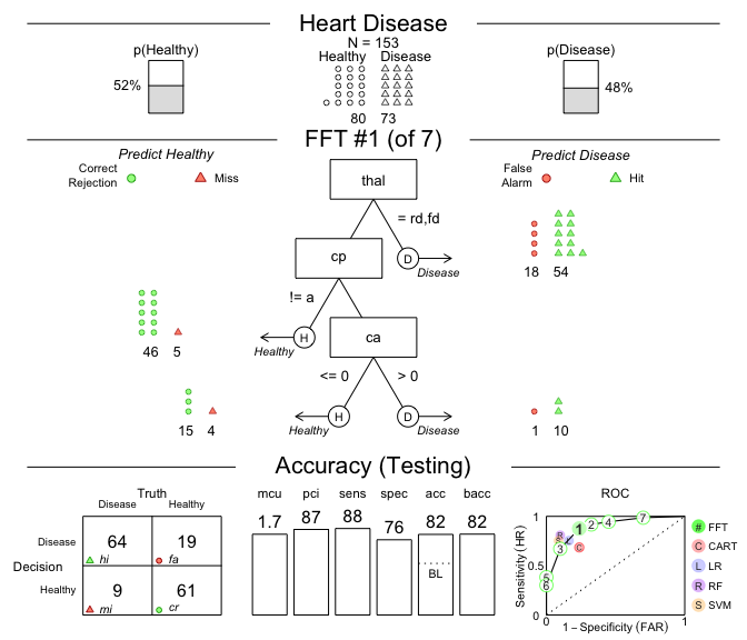
FFTrees object to visualize a tree and
its predictive performance (on the test data):# Plot the best tree applied to the test data:
plot(heart_fft,
data = "test",
main = "Heart Disease")
Figure 1: A fast-and-frugal tree (FFT) predicting
heart disease for test data and its performance
characteristics.
FFTrees object and their
key performance statistics can be obtained by
summary(heart_fft).FFTs are so simple that we even can create them ‘from words’ and then
apply them to data.
For example, let’s create a tree with the following three nodes and
evaluate its performance on the heart.test data:
sex = 1, predict Disease.age < 45, predict Healthy.thal = {fd, normal}, predict Healthy,These conditions can directly be supplied to the my.tree
argument of FFTrees():
# Create custom FFT 'in words' and apply it to test data:

# 1. Create my own FFT (from verbal description):
my_fft <- FFTrees(formula = diagnosis ~.,
                  data = heart.train,
                  data.test = heart.test,
                  decision.labels = c("Healthy", "Disease"),
                  my.tree = "If sex = 1, predict Disease.
                             If age < 45, predict Healthy.
                             If thal = {fd, normal}, predict Healthy,
                             Otherwise, predict Disease.")

# 2. Plot and evaluate my custom FFT (for test data):
plot(my_fft,
     data = "test",
     main = "My custom FFT")
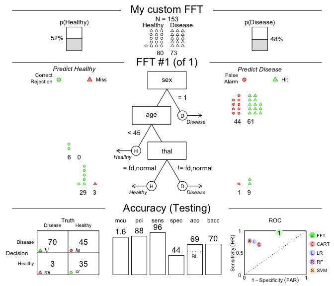
Figure 2: An FFT predicting heart disease created from a verbal description.
The performance measures (in the bottom panel of
Figure 2) show that this particular tree is somewhat
biased: It has nearly perfect sensitivity (i.e., is good at
identifying cases of Disease) but suffers from low
specificity (i.e., performs poorly in identifying
Healthy cases). Expressed in terms of its errors,
my_fft incurs few misses at the expense of many false
alarms. Although the accuracy of our custom tree still exceeds
the data’s baseline by a fair amount, the FFTs in heart_fft
(created above) strike a better balance.
Overall, what counts as the “best” tree for a particular problem depends on many factors (e.g., the goal of fitting vs. predicting data and the trade-offs between maximizing accuracy vs. incorporating the costs of cues or errors). To explore this range of options, the FFTrees package enables us to design and evaluate a range of FFTs.
The following versions of FFTrees and corresponding resources are available:
| Type: | Version: | URL: |
|---|---|---|
| A. FFTrees (R package): | Release version | https://CRAN.R-project.org/package=FFTrees |
| Development version | https://github.com/ndphillips/FFTrees | |
| B. Other resources: | Online documentation | https://www.nathanieldphillips.co/FFTrees/ |
| Online demo (running v1.3.3) | https://econpsychbasel.shinyapps.io/shinyfftrees/ |
We had fun creating the FFTrees package and hope you like it too! As a comprehensive, yet accessible introduction to FFTs, we recommend our article in the journal Judgment and Decision Making (2017), entitled FFTrees: A toolbox to create, visualize,and evaluate fast-and-frugal decision trees (available in html | PDF ).
Citation (in APA format):
We encourage you to read the article to learn more about the history of FFTs and how the FFTrees package creates, visualizes, and evaluates them. When using FFTrees in your own work, please cite us and share your experiences (e.g., on GitHub) so we can continue developing the package.
By 2025, over 150 scientific publications have used or cited FFTrees (see Google Scholar for the full list). Examples include:
Lötsch, J., Haehner, A., & Hummel, T. (2020). Machine-learning-derived rules set excludes risk of Parkinson’s disease in patients with olfactory or gustatory symptoms with high accuracy. Journal of Neurology, 267(2), 469–478. doi 10.1007/s00415-019-09604-6
Kagan, R., Parlee, L., Beckett, B., Hayden, J. B., Gundle, K. R., & Doung, Y. C. (2020). Radiographic parameter-driven decision tree reliably predicts aseptic mechanical failure of compressive osseointegration fixation. Acta Orthopaedica, 91(2), 171–176. doi 10.1080/17453674.2020.1716295
Klement, R. J., Sonke, J. J., Allgäuer, M., Andratschke, N., Appold, S., Belderbos, J., … & Mantel, F. (2020). Correlating dose variables with local tumor control in stereotactic body radiotherapy for early stage non-small cell lung cancer: A modeling study on 1500 individual treatments. International Journal of Radiation Oncology * Biology * Physics. doi 10.1016/j.ijrobp.2020.03.005
Nobre, G. G., Hunink, J. E., Baruth, B., Aerts, J. C., & Ward, P. J. (2019). Translating large-scale climate variability into crop production forecast in Europe. Scientific Reports, 9(1), 1–13. doi 10.1038/s41598-018-38091-4
Buchinsky, F. J., Valentino, W. L., Ruszkay, N., Powell, E., Derkay, C. S., Seedat, R. Y., … & Mortelliti, A. J. (2019). Age at diagnosis, but not HPV type, is strongly associated with clinical course in recurrent respiratory papillomatosis. PloS One, 14(6). doi 10.1371/journal.pone.0216697
[File README.Rmd last updated on 2025-09-03.]
These binaries (installable software) and packages are in development.
They may not be fully stable and should be used with caution. We make no claims about them.
Health stats visible at Monitor.