The hardware and bandwidth for this mirror is donated by dogado GmbH, the Webhosting and Full Service-Cloud Provider. Check out our Wordpress Tutorial.
If you wish to report a bug, or if you are interested in having us mirror your free-software or open-source project, please feel free to contact us at mirror[@]dogado.de.

This package provides code for estimating the combined toxicity of measured pesticides using their Species Sensitivity Distributions (SSDs) in a multi-substance, potentially affected fraction approach. The resulting value is an estimate of the percentage of species impacted by the measured pesticides; a value which is referred to in this package as the Pesticide Risk Metric (PRM). This is based on the Queensland Department of Environment and Science Water Quality & Investigation’s method used in the Reef 2050 Water Quality Improvement Plan. The main difference is the ability to add different pesticides to be measured provided they have one of the following SSD distributions:
These PRM values can be compared to the three categories of ecosystem condition, as defined in the Australian and New Zealand Guidelines for Fresh & Marine Water Quality seen in the table below.

The easiest way to install this package is from CRAN
install.packages("CalcThemAll.PRM")You can install the development version of CalcThemAll.PRM from GitHub with:
# install.packages("devtools")
devtools::install_github("AlexWaterboyBezzina/CalcThemAll.PRM")The process for calculating PRM estimates using this method is split into 4 main parts/functions:
add_your_own_pesticide()treat_LORs_all_data()calculate_daily_average_PRM()calculate_wet_season_average_PRM()An example of how to run this package is provided below using the
included Canto_pesticides concentration data.
library(CalcThemAll.PRM)
#1.Add new pesticides to pesticide_info table
pesticide_info <- add_your_own_pesticide(pesticides = #adding multiple new pesticides
                                           c("Poison", "Acid", "Sludge"),
                                         relative_LORs = c(0.03, 0.01, 0.5),
                                         pesticide_types = c("Ghost", "Bug", "Poison"),
                                         distribution_types = c("Log-Normal", "Log-Logistic
                                                                Log-Logistic", "Burr Type III"),
                                         scales = c(0.3, 0.002, 2),
                                         scale_2s = c(NA, 0.04, NA),
                                         shape_locations = c(1, 0.07, 3),
                                         shape_location_2s = c(NA, 0.14, 2.3),
                                         weights = c(NA, 0.08, NA))

#2.Treat LOR Values
Canto_pesticides_LOR_treated <- treat_LORs_all_data(raw_data = Canto_pesticides,
pesticide_info = CalcThemAll.PRM::pesticide_info, treatment_method = "WQI")

#3.Calculate Daily Average PRM
Canto_daily_PRM <- calculate_daily_average_PRM(LOR_treated_data = Canto_pesticides_LOR_treated)
head(Canto_daily_PRM)
#> # A tibble: 6 × 7
#>   `Site Name`    `Sampling Year` Date       `Total PRM` `Insecticide PRM`
#>   <chr>          <chr>           <chr>            <dbl>             <dbl>
#> 1 Celestial City 2017-2018       2017-07-03       22.9      0.000126
#> 2 Celestial City 2017-2018       2017-07-10        7.34     0.0000172
#> 3 Celestial City 2017-2018       2017-07-18       47.0      0.0145
#> 4 Celestial City 2017-2018       2017-07-24       14.6      0.00851
#> 5 Celestial City 2017-2018       2017-07-30       17.2      0.00533
#> 6 Celestial City 2017-2018       2017-08-08        5.28     0.00000000193
#> # ℹ 2 more variables: `Other Herbicide PRM` <dbl>, `PSII Herbicide PRM` <dbl>

Violet_Town_2017_2018_PRM <- Canto_daily_PRM %>%
 dplyr::filter(.data$`Sampling Year` ==  "2017-2018" &  .data$`Site Name` == "Violet Town")

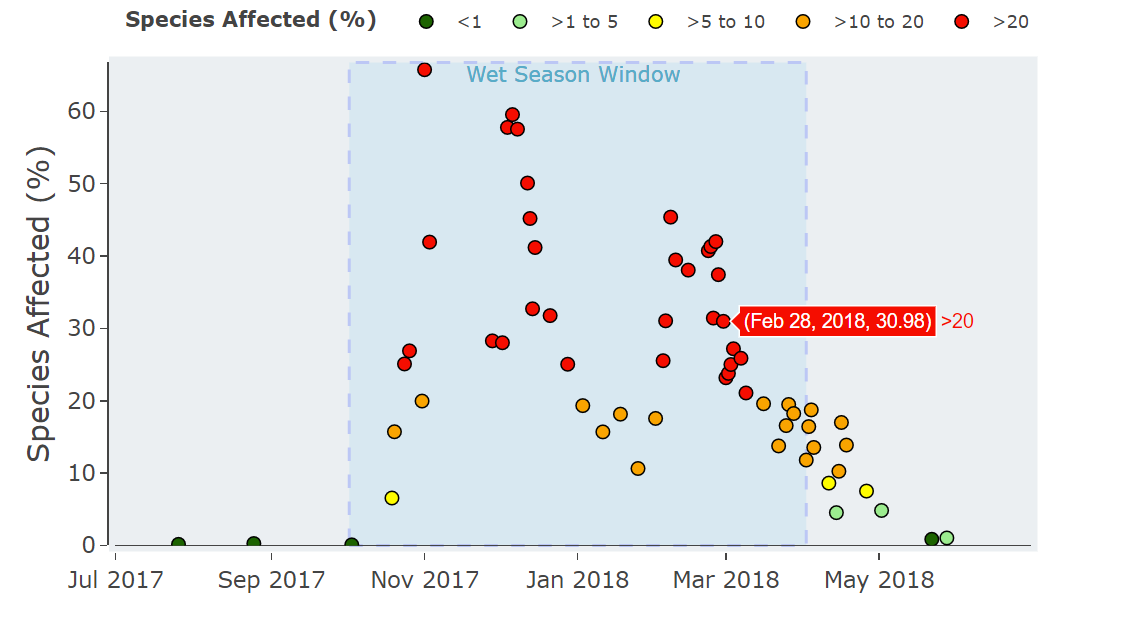
plot <- plot_daily_PRM(daily_PRM_data = Violet_Town_2017_2018_PRM,
               wet_season_start = "2017-10-02", #start date of the wet season or high risk window
                                                #this is optional and can be removed with = NULL
               wet_season_length = 182, #length of wet season or high risk window
               PRM_group = "PSII Herbicide PRM") #PRM group to plot, for all PRM = "Total PRM
#4.Calculate Wet Season Average PRM
Celestial_City_2019_2020_daily_PRM <- Canto_daily_PRM %>%
  dplyr::filter(`Site Name` == "Celestial City" & `Sampling Year` == "2019-2020")
#This calculation can take a few minutes so one site & sampling year is used in this example

CC2019_2020_wet_season_Total_PRM <- calculate_wet_season_average_PRM(daily_PRM_data = Celestial_City_2019_2020_daily_PRM, PRM_group = "Total PRM")
#this calculates the wet season average PRM for all pesticide groups in one total value
#to calculate for a specific group define it in "PRM_group ="

CC2019_2020_wet_season_Total_PRM
#> # A tibble: 1 × 3
#>   `Site Name`    `Sampling Year` `Total PRM`
#>   <chr>          <chr>                 <dbl>
#> 1 Celestial City 2019-2020 26.7Information is from several sources and, as such, does not necessarily represent government or departmental policy. While every care is taken to ensure the accuracy of this information, the Department of Environment and Science makes no representations or warranties relating to accuracy, reliability, completeness, currency or suitability for any particular purpose and disclaims all responsibility and all liability (including without limitation, liability in negligence) for all expenses, losses, damages (including indirect or consequential damage) and costs that might be incurred as a result of any use or of reliance on the information and calculated data in any way and for any reason.
R Package:
Bezzina A, Neelamraju C, Strauss J, Kaminski H, Roberts C, Glen J, Dias F. 2022. CalcThemAll.PRM: Pesticide Risk Metric Calculations. R package. Water Quality Monitoring & Investigations, Department of Environment and Science, Queensland Government. https://github.com/AlexWaterboyBezzina/CalcThemAll.PRM
Methods Behind Pesticide Risk Metric:
Warne MStJ, Neelamraju C, Strauss J, Smith RA, Turner RDR, Mann RM. 2020. Development of a method for estimating the toxicity of pesticide mixtures and a Pesticide Risk Baseline for the Reef 2050 Water Quality Improvement Plan. Brisbane: Department of Environment and Science, Queensland Government.
These binaries (installable software) and packages are in development.
They may not be fully stable and should be used with caution. We make no claims about them.
Health stats visible at Monitor.