The hardware and bandwidth for this mirror is donated by dogado GmbH, the Webhosting and Full Service-Cloud Provider. Check out our Wordpress Tutorial.
If you wish to report a bug, or if you are interested in having us mirror your free-software or open-source project, please feel free to contact us at mirror[@]dogado.de.

BayesSurvive

This is a R/Rcpp package BayesSurvive for Bayesian survival models with graph-structured selection priors for sparse identification of high-dimensional features predictive of survival (Hermansen et al., 2025; Madjar et al., 2021) (see the three models of the first column in the table below) and its extensions with the use of a fixed graph via a Markov Random Field (MRF) prior for capturing known structure of high-dimensional features (see the three models of the second column in the table below), e.g. disease-specific pathways from the Kyoto Encyclopedia of Genes and Genomes (KEGG) database.

Installation

Install the latest released version from CRAN

install.packages("BayesSurvive")

Install the latest development version from GitHub

#install.packages("remotes")
remotes::install_github("ocbe-uio/BayesSurvive")

Examples

Simulate data

library("BayesSurvive")
# Load the example dataset
data("simData", package = "BayesSurvive")
dataset = list("X" = simData[[1]]$X, 
               "t" = simData[[1]]$time,
               "di" = simData[[1]]$status)

Run a Bayesian Cox model

## Initial value: null model without covariates
initial = list("gamma.ini" = rep(0, ncol(dataset$X)))
# Prior parameters
hyperparPooled = list(
  "c0"     = 2,                      # prior of baseline hazard
  "tau"    = 0.0375,                 # sd (spike) for coefficient prior
  "cb"     = 20,                     # sd (slab) for coefficient prior
  "pi.ga"  = 0.02,                   # prior variable selection probability for standard Cox models
  "a"      = -4,                     # hyperparameter in MRF prior
  "b"      = 0.1,                    # hyperparameter in MRF prior
  "G"      = simData$G               # hyperparameter in MRF prior
)   

## run Bayesian Cox with graph-structured priors
set.seed(123)
fit <- BayesSurvive(survObj = dataset, model.type = "Pooled", MRF.G = TRUE, 
                    hyperpar = hyperparPooled, initial = initial, 
                    nIter = 200, burnin = 100)

## show posterior mean of coefficients and 95% credible intervals
library("GGally")
plot(fit) + 
  coord_flip() + 
  theme(axis.text.x = element_text(angle = 90, size = 7))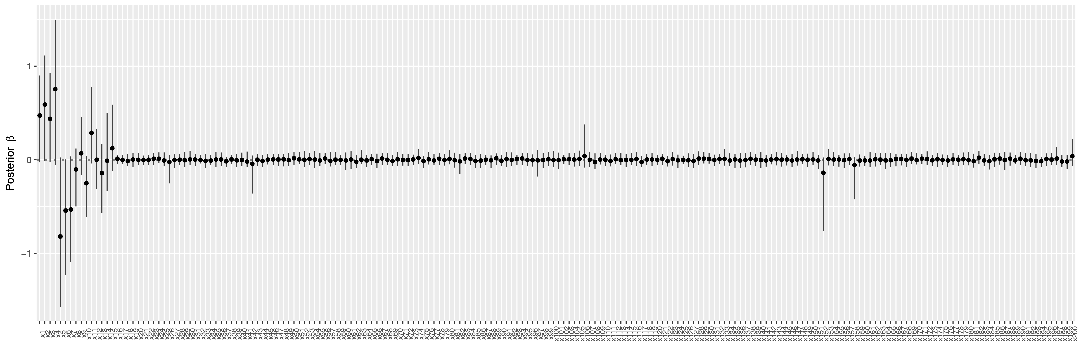

Show the index of selected variables by controlling Bayesian false discovery rate (FDR) at the level \(\alpha = 0.05\)

which( VS(fit, method = "FDR", threshold = 0.05) )

#[1]   1   2   3   4   5   6   7   8   9  10  11  12  13  14  15 128

Plot time-dependent Brier scores

The function BayesSurvive::plotBrier() can show the time-dependent Brier scores based on posterior mean of coefficients or Bayesian model averaging.

plotBrier(fit, survObj.new = dataset)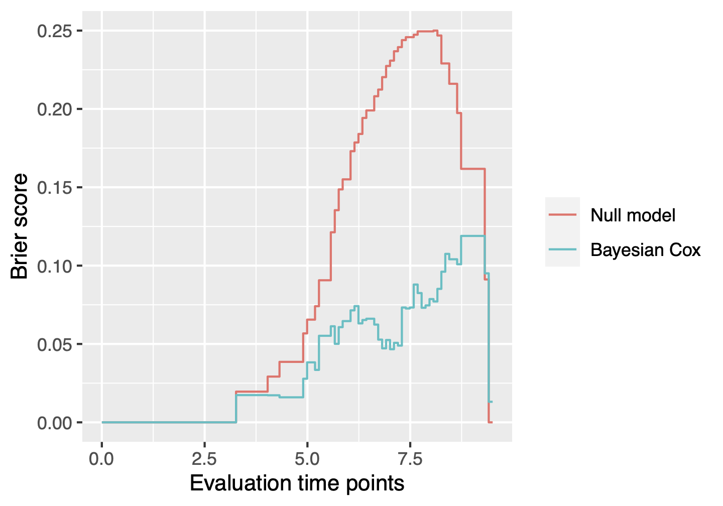

We can also use the function BayesSurvive::predict() to obtain the Brier score at time 8.5, the integrated Brier score (IBS) from time 0 to 8.5 and the index of prediction accuracy (IPA).

predict(fit, survObj.new = dataset, times = 8.5)

##               Brier(t=8.5) IBS(t:0~8.5) IPA(t=8.5)
## Null.model      0.2290318   0.08185316  0.0000000
## Bayesian.Cox    0.1037802   0.03020026  0.5468741

Predict survival probabilities and cumulative hazards

The function BayesSurvive::predict() can estimate the survival probabilities and cumulative hazards.

predict(fit, survObj.new = dataset, type = c("cumhazard", "survival"))

#        observation times cumhazard  survival
##              <int> <num>     <num>     <num>
##     1:           1   3.3  1.04e-04 1.00e+00
##     2:           2   3.3  3.88e-01 6.78e-01
##     3:           3   3.3  1.90e-06 1.00e+00
##     4:           4   3.3  1.94e-03 9.98e-01
##     5:           5   3.3  4.08e-04 1.00e+00
##    ---                                     
##  9996:          96   9.5  1.40e+01 8.21e-07
##  9997:          97   9.5  8.25e+01 1.45e-36
##  9998:          98   9.5  5.37e-01 5.85e-01
##  9999:          99   9.5  2.00e+00 1.35e-01
## 10000:         100   9.5  3.58e+00 2.79e-02

Run a ‘Pooled’ Bayesian Cox model with graphical learning

hyperparPooled <- append(hyperparPooled, list("lambda" = 3, "nu0" = 0.05, "nu1" = 5))
fit2 <- BayesSurvive(survObj = list(dataset), model.type = "Pooled", MRF.G = FALSE,
                     hyperpar = hyperparPooled, initial = initial, nIter = 10)

Run a Bayesian Cox model with subgroups using fixed graph

# specify a fixed joint graph between two subgroups
hyperparPooled$G <- Matrix::bdiag(simData$G, simData$G)
dataset2 <- simData[1:2]
dataset2 <- lapply(dataset2, setNames, c("X", "t", "di", "X.unsc", "trueB"))
fit3 <- BayesSurvive(survObj = dataset2, 
                     hyperpar = hyperparPooled, initial = initial, 
                     model.type="CoxBVSSL", MRF.G = TRUE, 
                     nIter = 10, burnin = 5)

Run a Bayesian Cox model with subgroups using graphical learning

fit4 <- BayesSurvive(survObj = dataset2, 
                     hyperpar = hyperparPooled, initial = initial, 
                     model.type="CoxBVSSL", MRF.G = FALSE, 
                     nIter = 3, burnin = 0)

References

Tobias Østmo Hermansen, Manuela Zucknick, Zhi Zhao (2025). Bayesian Cox model with graph-structured variable selection priors for multi-omics biomarker identification. arXiv. DOI: arXiv.2503.13078.

Katrin Madjar, Manuela Zucknick, Katja Ickstadt, Jörg Rahnenführer (2021). Combining heterogeneous subgroups with graph‐structured variable selection priors for Cox regression. BMC Bioinformatics, 22(1):586. DOI: 10.1186/s12859-021-04483-z.

These binaries (installable software) and packages are in development.
They may not be fully stable and should be used with caution. We make no claims about them.
Health stats visible at Monitor.