The hardware and bandwidth for this mirror is donated by dogado GmbH, the Webhosting and Full Service-Cloud Provider. Check out our Wordpress Tutorial.
If you wish to report a bug, or if you are interested in having us mirror your free-software or open-source project, please feel free to contact us at mirror[@]dogado.de.
BayesGrowth combines length-at-age modelling for fisheries with MCMC
implemented using Stan and the rstan package.
Growth modelling using models such as the von Bertalanffy growth model
involves three parameters: , k and either
or
. Two of these parameters:
and
have direct biological meaning as the size-at-birth and
maximum length, respectively. This package provides the tools to run an
MCMC model with these two parameters treated as size-at-birth and
maximum length using a rstan model with a No U-Turn Sampling (NUTS)
algorithm. This MCMC model is pre-specified and built into wrapper
functions.
The user can therefore run an MCMC growth model using knowledge of species length-at-birth and maximum size as priors.
You can install the released version of BayesGrowth from Github using devtools. There is a vignette that runs an example and demonstrates how to examine diagnostic plots.
if (!require("devtools")) {
  install.packages("devtools")
}

devtools::install_github("jonathansmart/BayesGrowth", build_vignettes = TRUE)

browseVignettes("BayesGrowth")
Or alternatively you can install the latest release manually. This can be useful as when downloading from github you’ll automatically build the package from the source. However, as the rstan models contain compiled code, this can lead to build errors without proper installs of devtools or Rtools.
If you need to install the package manually (skipping the compiling) you can go to the latest release and download the package file (‘BayesGrowth_ver.zip’). This can then be installed from Rstudio using Packages -> Install -> Package Archive File (.zip, tar.gz).
The main BayesGrowth function is
Estimate_MCMC_Growth which is the wrapper function around
an rstan model. It requires a data input that includes columns that can
be identified “Age” and “Length”, the model needs to be specified
(several options are available) and the priors must be specified. Priors
include the max size with an error, length-at-birth with an error and
upper limits for k and .
These latter two parameters have no informative priors and only require
sensible upper bounds. Many fish species (including this example) have a
size at birth of zero. Therefore, this can value can be used as a prior
along with a very small error to indicate high certainty of this prior.
The
L0.se argument cannot be zero, but the model is
specified to truncate at zero and keep growth positive.
library(BayesGrowth)

data("example_data")

## Biological info - lengths in mm
max_size <- 440
max_size_se <- 5
birth_size <- 0
birth_size_se <- 0.001 # an se cannot be zero

# Use the function to estimate the rstan model
fit <- Estimate_MCMC_Growth(data = example_data,
                            Model = "VB" ,
                            iter = 5000,
                            Linf = max_size,
                            Linf.se = max_size_se,
                            L0 = birth_size,
                            sigma.max = 100,
                            L0.se = birth_size_se,
                            k.max = 1)
The function returns the rstan outputs which is an object of class “stanfit”
fit
#> Inference for Stan model: VB_stan_model.
#> 4 chains, each with iter=5000; warmup=2500; thin=1;
#> post-warmup draws per chain=2500, total post-warmup draws=10000.
#>
#>           mean se_mean   sd     2.5%      25%      50%      75%    97.5% n_eff
#> Linf    317.86    0.09 4.13   310.52   314.98   317.58   320.40   326.58  2150
#> k         0.66    0.00 0.03     0.59     0.64     0.66     0.69     0.73  2274
#> L0        0.00    0.00 0.00     0.00     0.00     0.00     0.00     0.00  3991
#> sigma    24.30    0.02 0.87    22.73    23.68    24.25    24.87    26.13  2538
#> lp__  -3933.95    0.03 1.52 -3937.81 -3934.70 -3933.61 -3932.84 -3932.06  2305
#>       Rhat
#> Linf     1
#> k        1
#> L0       1
#> sigma    1
#> lp__     1
#>
#> Samples were drawn using NUTS(diag_e) at Mon Nov 20 13:44:46 2023.
#> For each parameter, n_eff is a crude measure of effective sample size,
#> and Rhat is the potential scale reduction factor on split chains (at
#> convergence, Rhat=1).
Therefore, all of the diagnostics from the rstan library can be used.
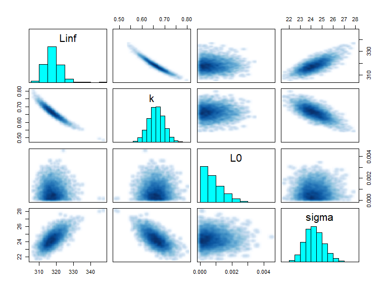
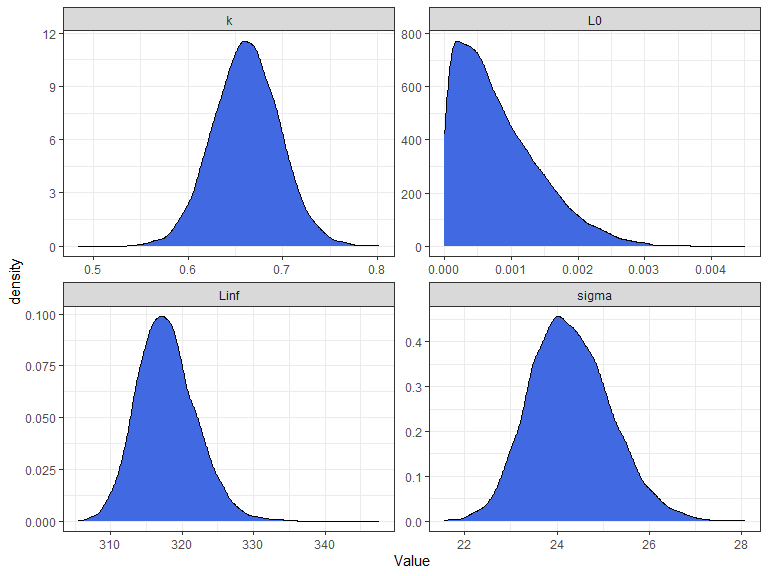
Some examples are the pairs and extract
functions:
library(tidyverse)
library(rstan)

pairs(fit, pars = c("Linf", "k","L0", "sigma"))
#> Warning in par(usr): argument 1 does not name a graphical parameter

#> Warning in par(usr): argument 1 does not name a graphical parameter

#> Warning in par(usr): argument 1 does not name a graphical parameter

#> Warning in par(usr): argument 1 does not name a graphical parameter
list_of_draws <- extract(fit,c("Linf", "k","L0", "sigma")) %>%
  as.data.frame() %>%
  gather(Parameter, Value) %>%
  filter(Parameter %in% c("Linf", "k","L0", "sigma"))


ggplot(list_of_draws, aes(Value))+
  geom_density(fill = "royalblue")+
  facet_wrap(~Parameter, scales = "free", ncol = 2)+
  theme_bw()
Additional BayesGrowth functions are available that help
the user manipulate the returned Estimate_MCMC_Growth
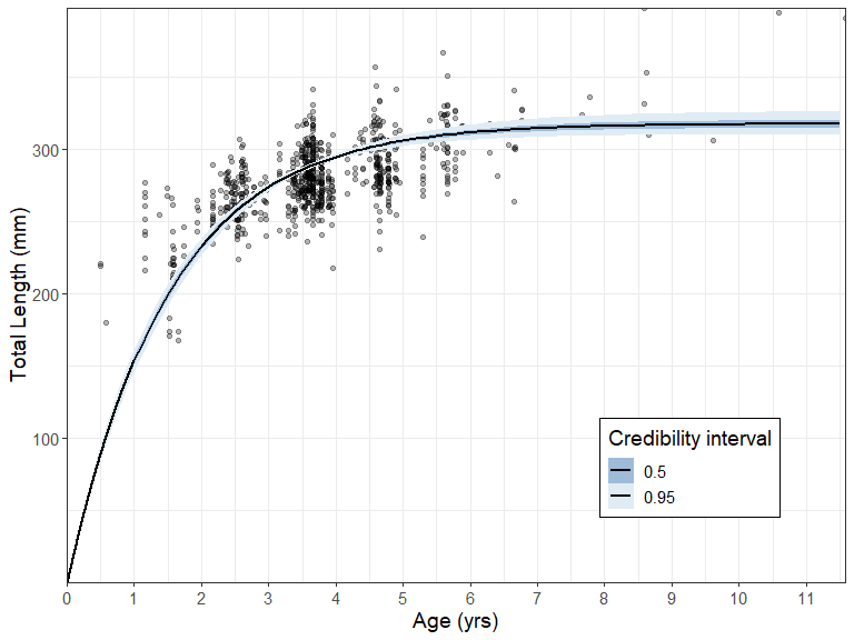
object. The Calculate_MCMC_growth_curve function will
provide confidence intervals around the growth curve based on MCMC
parameter percentiles. This is essentially a wrapper around the
tidybayes::mean_qi() function which means it can be passed
straight into a ggplot with the tidybayes::geom_line_ribbon
function.
library(tidybayes)

# Return a growth curve with 50th and 95th percentiles
growth_curve <- Calculate_MCMC_growth_curve(fit, Model = "VB",
                                            max.age = max(example_data$Age), probs = c(.5,.95))


ggplot(growth_curve, aes(Age, LAA))+
  geom_point(data = example_data, aes(Age, Length), alpha = .3)+
  geom_lineribbon(aes( ymin = .lower, ymax = .upper, fill = factor(.width)), size = .8) +
  labs(y = "Total Length (mm)", x = "Age (yrs)")+
  scale_fill_brewer(palette="BuPu", direction=-1,name = "Credibility interval")+
  scale_y_continuous(expand = c(0,0))+
  scale_x_continuous(expand = c(0,0), breaks = seq(0,13,1))+
  theme_bw()+
  theme(text = element_text(size = 14),
        legend.position = c(0.8,0.2),
        legend.background = element_rect(colour = "black"))
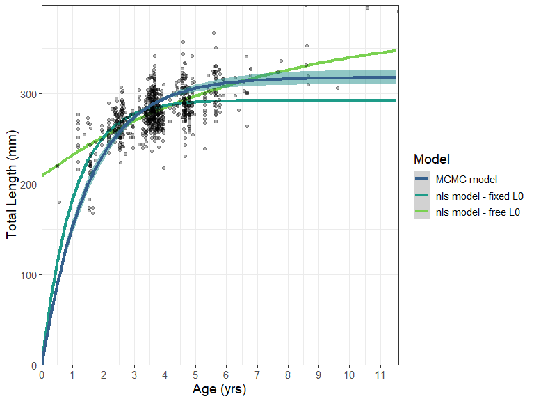
This represents a much improved fit over a standard non-linear estimated model, even if the length-at-birth were fixed at zero. Here the fit is compared using an nls model fit using the AquaticLifeHistory package.

These binaries (installable software) and packages are in development.
They may not be fully stable and should be used with caution. We make no claims about them.
Health stats visible at Monitor.