The hardware and bandwidth for this mirror is donated by dogado GmbH, the Webhosting and Full Service-Cloud Provider. Check out our Wordpress Tutorial.
If you wish to report a bug, or if you are interested in having us mirror your free-software or open-source project, please feel free to contact us at mirror[@]dogado.de.
![]()
![]()
BayesERtools provides a suite of tools that facilitate
exposure-response analysis using Bayesian methods.
BayesERbook): https://genentech.github.io/BayesERbook/You can install the BayesERtools with:
install.packages('BayesERtools')
# devtools::install_github("genentech/BayesERtools") # development version|
Binary endpoint
|
Continuous endpoint
|
|||
|---|---|---|---|---|
| Linear (logit) | Emax (logit) | Linear | Emax | |
| backend |
rstanarm
|
rstanemax
|
rstanarm
|
rstanemax
|
| reference | 🔗 | 🔗 | 🔗 | 🔗 |
| develop model | ✅ | ✅ | ✅ | ✅ |
| simulate & plot ER | ✅ | ✅ | ✅ | ✅ |
| exposure metrics selection | ✅ | ✅ | ✅ | ✅ |
| covariate selection | ✅ | ❌ | ✅ | ❌ |
| covariate forest plot | ✅ | ❌ | ✅ | ❌ |
| ✅ Available, 🟡 In plan/under development, ❌ Not in a current plan | ||||
Here is a quick demo on how to use this package for E-R analysis. See Basic workflow for more thorough walk through.
# Load package and data
library(dplyr)
library(BayesERtools)
theme_set(theme_bw(base_size = 12))

data(d_sim_binom_cov)

# Hyperglycemia Grade 2+ (hgly2) data
df_er_ae_hgly2 <-
  d_sim_binom_cov |>
  filter(AETYPE == "hgly2") |>
  # Re-scale AUCss, baseline age
  mutate(
    AUCss_1000 = AUCss / 1000, BAGE_10 = BAGE / 10,
    Dose = paste(Dose_mg, "mg")
  )

var_resp <- "AEFLAG"set.seed(1234)
ermod_bin <- dev_ermod_bin(
data = df_er_ae_hgly2,
var_resp = var_resp,
var_exposure = "AUCss_1000"
)
ermod_bin
#>
#> ── Binary ER model ─────────────────────────────────────────────────────────────
#> ℹ Use `plot_er()` to visualize ER curve
#>
#> ── Developed model ──
#>
#> stan_glm
#> family: binomial [logit]
#> formula: AEFLAG ~ AUCss_1000
#> observations: 500
#> predictors: 2
#> ------
#> Median MAD_SD
#> (Intercept) -2.04 0.23
#> AUCss_1000 0.41 0.08
#> ------
#> * For help interpreting the printed output see ?print.stanreg
#> * For info on the priors used see ?prior_summary.stanreg
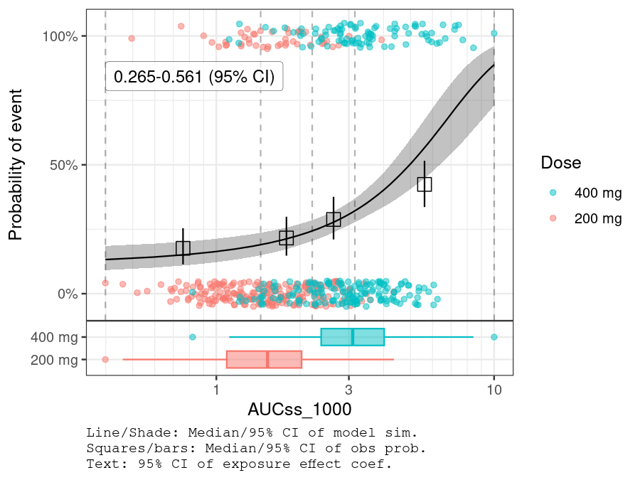
# Using `*` instead of `+` so that scale can be
# applied for both panels (main plot and boxplot)
plot_er_gof(ermod_bin, var_group = "Dose", show_coef_exp = TRUE) *
coord_transform(x = "log10") *
scale_x_continuous(
breaks = xgxr::xgx_breaks_log10,
minor_breaks = xgxr::xgx_minor_breaks_log10
)
BGLUC (baseline glucose) is selected while other two covariates are not.
set.seed(1234)
ermod_bin_cov_sel <-
  dev_ermod_bin_cov_sel(
    data = df_er_ae_hgly2,
    var_resp = var_resp,
    var_exposure = "AUCss_1000",
    var_cov_candidate = c("BAGE_10", "RACE", "BGLUC")
  )
#>
#> ── Step 1: Full reference model fit ──
#>
#> ── Step 2: Variable selection ──
#>
#> ℹ The variables selected were: AUCss_1000, BGLUC
#>
#> ── Step 3: Final model fit ──
#>
#> ── Cov mod dev complete ──
#>
ermod_bin_cov_sel
#> ── Binary ER model & covariate selection ───────────────────────────────────────
#> ℹ Use `plot_submod_performance()` to see variable selection performance
#> ℹ Use `plot_er()` with `marginal = TRUE` to visualize marginal ER curve
#>
#> ── Selected model ──
#>
#> stan_glm
#>  family:       binomial [logit]
#>  formula:      AEFLAG ~ AUCss_1000 + BGLUC
#>  observations: 500
#>  predictors:   3
#> ------
#>             Median MAD_SD
#> (Intercept) -7.59   0.90
#> AUCss_1000   0.46   0.08
#> BGLUC        0.87   0.13
#> ------
#> * For help interpreting the printed output see ?print.stanreg
#> * For info on the priors used see ?prior_summary.stanreg
plot_submod_performance(ermod_bin_cov_sel)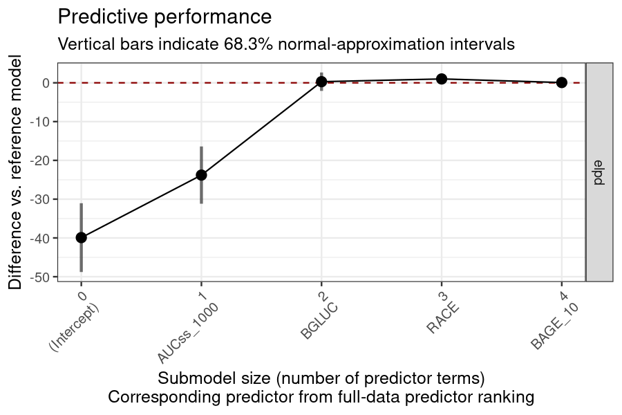
coveffsim <- sim_coveff(ermod_bin_cov_sel)
plot_coveff(coveffsim)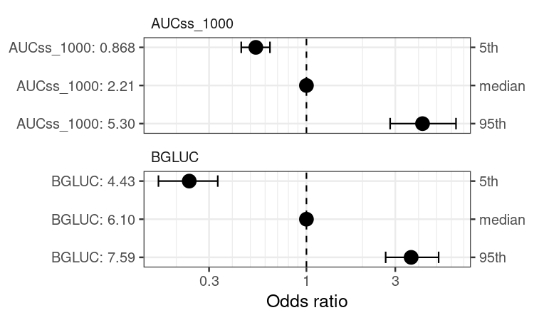
These binaries (installable software) and packages are in development.
They may not be fully stable and should be used with caution. We make no claims about them.
Health stats visible at Monitor.