The hardware and bandwidth for this mirror is donated by dogado GmbH, the Webhosting and Full Service-Cloud Provider. Check out our Wordpress Tutorial.
If you wish to report a bug, or if you are interested in having us mirror your free-software or open-source project, please feel free to contact us at mirror[@]dogado.de.
Bayesian Spatial Blind Source Separation via Thresholded Gaussian Process.
Install the released version of BSPBSS from Github with:
devtools::install_github("benwu233/BSPBSS")This is a basic example which shows you how to solve a common problem.
First we load the package and generate simulated images with a probabilistic ICA model:
library(BSPBSS)
set.seed(612)
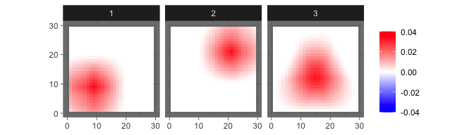
sim = sim_2Dimage(length = 30, sigma = 5e-4, n = 30, smooth = 6)The true source signals are three 2D geometric patterns (set
smooth=0 to generate patterns with sharp edges).
levelplot2D(sim$S,lim = c(-0.04,0.04), sim$coords)
which generate observed images such as
levelplot2D(sim$X[1:3,], lim = c(-0.12,0.12), sim$coords)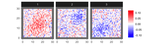
Then we generate initial values for mcmc,
ini = init_bspbss(sim$X, sim$coords, q = 3, ker_par = c(0.1,50), num_eigen = 50)and run!
res = mcmc_bspbss(ini$X,ini$init,ini$prior,ini$kernel,n.iter=2000,n.burn_in=1000,thin=10,show_step=1000)
#> iter 1000 Sat Oct  1 22:12:33 2022
#>
#>  stepsize_zeta 0.0167947 accp_rate_zeta 0.34
#> iter 2000 Sat Oct  1 22:12:36 2022
#>
#>  stepsize_zeta 0.0167947 accp_rate_zeta 0.37
Then the results can be summarized by
res_sum = sum_mcmc_bspbss(res, ini$X, ini$kernel, start = 101, end = 200, select_p = 0.5)and shown by
levelplot2D(res_sum$S, lim = c(-1.3,1.3), sim$coords)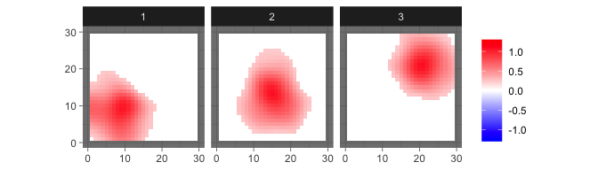
For comparison, we show the estimated sources provided by informax ICA here.
levelplot2D(ini$init$ICA_S, lim = c(-1.7,1.7), sim$coords)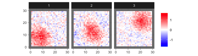
We may overspecify the number of components and still obtain reasonable results.
ini = init_bspbss(sim$X, sim$coords, q = 5, ker_par = c(0.1,50), num_eigen = 50)
res = mcmc_bspbss(ini$X,ini$init,ini$prior,ini$kernel, n.iter=2000,n.burn_in=1000,thin=10,show_step=1000)
#> iter 1000 Sat Oct  1 22:12:40 2022
#>
#>  stepsize_zeta 0.0104649 accp_rate_zeta 0.35
#> iter 2000 Sat Oct  1 22:12:43 2022
#>
#>  stepsize_zeta 0.0104649 accp_rate_zeta 0.43
res_sum = sum_mcmc_bspbss(res, ini$X, ini$kernel, start = 101, end = 200, select_p = 0.5)
levelplot2D(res_sum$S, lim = c(-1.3,1.3), sim$coords)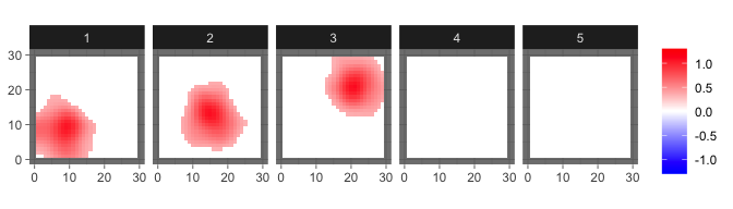
Install a small pack contains simulated NIfTI images and MNI152 template.
devtools::install_github("benwu233/SIMDATA")Load and take a glance at the data.
data_path = system.file("extdata",package="SIMDATA")
t1_3mm = neurobase::readNIfTI2(paste0(data_path,"/template/MNI152_T1_3mm.nii.gz"))
sim_4d = neurobase::readNIfTI2(paste0(data_path,"/sim_4d/sim_4d.nii.gz"))
mask = neurobase::readNIfTI2(paste0(data_path,"/sim_4d/mask.nii.gz"))
neurobase::ortho2(t1_3mm, y=sim_4d[,,,1])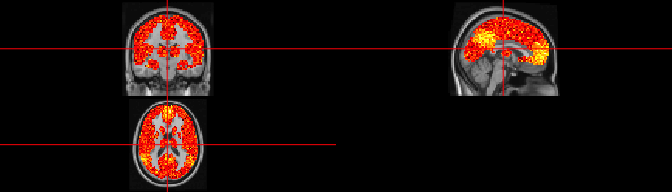
Conduct BSPBSS.
X = pre_nii(sim_4d,mask)
ini = init_bspbss(X$data, X$coords, dens = 0.5, q = 3, ker_par = c(0.01, 120), num_eigen = 200)
res = mcmc_bspbss(ini$X,ini$init,ini$prior,ini$kernel,n.iter=3000,n.burn_in=2000,thin=10,show_step=1000,subsample_p=0.005)
#> iter 1000 Sat Oct  1 22:14:38 2022
#>
#>  stepsize_zeta 0.00296575 accp_rate_zeta 0.42
#> iter 2000 Sat Oct  1 22:16:28 2022
#>
#>  stepsize_zeta 0.00769239 accp_rate_zeta 0.42
#> iter 3000 Sat Oct  1 22:18:19 2022
#>
#>  stepsize_zeta 0.00769239 accp_rate_zeta 0.41
res_sum = sum_mcmc_bspbss(res, ini$X, ini$kernel, start = 201, end = 300, select_p = 0.5)
Output:
ICs = output_nii(res_sum$S,sim_4d,X$coords,file=NULL,std=TRUE)Component 1:
neurobase::ortho2(t1_3mm,y=ICs[,,,1])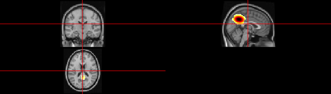 Component 2:
neurobase::ortho2(t1_3mm,y=ICs[,,,2])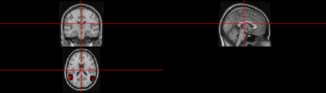 Component 3:
neurobase::ortho2(t1_3mm,y=ICs[,,,3])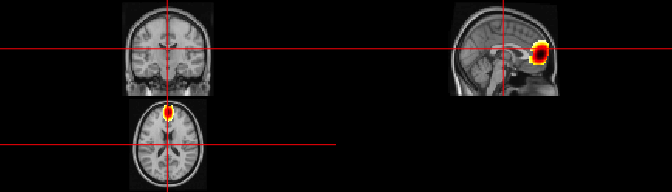
These binaries (installable software) and packages are in development.
They may not be fully stable and should be used with caution. We make no claims about them.
Health stats visible at Monitor.