The hardware and bandwidth for this mirror is donated by dogado GmbH, the Webhosting and Full Service-Cloud Provider. Check out our Wordpress Tutorial.
If you wish to report a bug, or if you are interested in having us mirror your free-software or open-source project, please feel free to contact us at mirror[@]dogado.de.
The goal of AssetAllocation is to perform backtesting of customizable asset allocation strategies. The main function that the user interacts with is backtest_allocation().
You can install the development version of AssetAllocation from GitHub with:
# install.packages("devtools")
devtools::install_github("rubetron/AssetAllocation")Simple example using pre-loaded strategy (see the vignette for other examples):
library(AssetAllocation)
#> Registered S3 method overwritten by 'quantmod':
#> method from
#> as.zoo.data.frame zoo
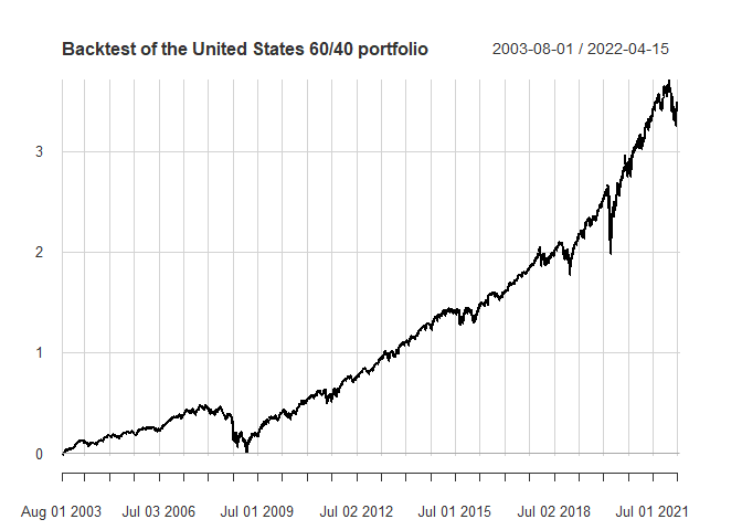
## Example 1: backtesting one of the asset allocations in the package
us_60_40 <- asset_allocations$static$us_60_40
# test using the data set provided in the package
bt_us_60_40 <- backtest_allocation(us_60_40,
ETFs$Prices,
ETFs$Returns,
ETFs$risk_free)
# plot returns
library(PerformanceAnalytics)
#> Loading required package: xts
#> Loading required package: zoo
#>
#> Attaching package: 'zoo'
#> The following objects are masked from 'package:base':
#>
#> as.Date, as.Date.numeric
#>
#> Attaching package: 'PerformanceAnalytics'
#> The following object is masked from 'package:graphics':
#>
#> legend
chart.CumReturns(bt_us_60_40$returns,
main = paste0("Backtest of the ",
bt_us_60_40$strat$name,
" portfolio"),
ylab = "Cumulative returns"
)
# show table with performance metrics
bt_us_60_40$table_performance
#>                               United.States.60.40
#> Annualized Return                          0.0803
#> Annualized Std Dev                         0.1013
#> Annualized Sharpe (Rf=1.18%)               0.6669
#> daily downside risk                        0.0045
#> Annualised downside risk                   0.0718
#> Downside potential                         0.0019
#> Omega                                      1.1466
#> Sortino ratio                              0.0618
#> Upside potential                           0.0022
#> Upside potential ratio                     0.6175
#> Omega-sharpe ratio                         0.1466
#> Semi Deviation                             0.0046
#> Gain Deviation                             0.0046
#> Loss Deviation                             0.0053
#> Downside Deviation (MAR=210%)              0.0100
#> Downside Deviation (Rf=1.18%)              0.0045
#> Downside Deviation (0%)                    0.0045
#> Maximum Drawdown                           0.3260
#> Historical VaR (95%)                      -0.0093
#> Historical ES (95%)                       -0.0155
#> Modified VaR (95%)                        -0.0086
#> Modified ES (95%)                         -0.0086
Another example creating a strategy from scratch, retrieving data from Yahoo Finance, and backtesting:
library(AssetAllocation)
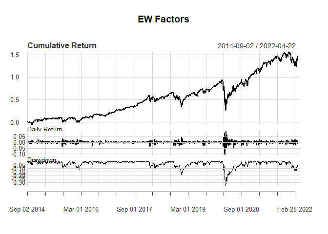
# create a strategy that invests equally in momentum (MTUM), value (VLUE), low volatility (USMV) and quality (QUAL) ETFs.
factors_EW <- list(name = "EW Factors",
tickers = c("MTUM", "VLUE", "USMV", "QUAL"),
default_weights = c(0.25, 0.25, 0.25, 0.25),
rebalance_frequency = "month",
portfolio_rule_fn = "constant_weights")
# get data for tickers using getSymbols
factor_ETFs_data <- get_data_from_tickers(factors_EW$tickers,
starting_date = "2013-08-01")
#> 'getSymbols' currently uses auto.assign=TRUE by default, but will
#> use auto.assign=FALSE in 0.5-0. You will still be able to use
#> 'loadSymbols' to automatically load data. getOption("getSymbols.env")
#> and getOption("getSymbols.auto.assign") will still be checked for
#> alternate defaults.
#>
#> This message is shown once per session and may be disabled by setting
#> options("getSymbols.warning4.0"=FALSE). See ?getSymbols for details.
# backtest the strategy
bt_factors_EW <- backtest_allocation(factors_EW,factor_ETFs_data$P, factor_ETFs_data$R)
# plot returns
charts.PerformanceSummary(bt_factors_EW$returns,
main = bt_factors_EW$strat$name,
)
# table with performance metrics
bt_factors_EW$table_performance
#>                               EW.Factors
#> Annualized Return                 0.1233
#> Annualized Std Dev                0.1731
#> Annualized Sharpe (Rf=0%)         0.7125
#> daily downside risk               0.0078
#> Annualised downside risk          0.1246
#> Downside potential                0.0032
#> Omega                             1.1652
#> Sortino ratio                     0.0664
#> Upside potential                  0.0037
#> Upside potential ratio            0.5665
#> Omega-sharpe ratio                0.1652
#> Semi Deviation                    0.0081
#> Gain Deviation                    0.0077
#> Loss Deviation                    0.0094
#> Downside Deviation (MAR=210%)     0.0125
#> Downside Deviation (Rf=0%)        0.0078
#> Downside Deviation (0%)           0.0078
#> Maximum Drawdown                  0.3499
#> Historical VaR (95%)             -0.0161
#> Historical ES (95%)              -0.0266
#> Modified VaR (95%)               -0.0151
#> Modified ES (95%)                -0.0168
These binaries (installable software) and packages are in development.
They may not be fully stable and should be used with caution. We make no claims about them.
Health stats visible at Monitor.