Chord identity and comparison
You have already seen is_chord, which is similar to is_note. Another check that can be performed on chords is whether they are diatonic to a scale. chord_is_diatonic strictly accepts chords in noteworthy strings.
#> [1] TRUE FALSE
A few functions that compare chords are chord_rank, chord_order and chord_sort. Ranking chords, and the ordering and sorting based on that, requires a definition or set of definitions to work from.
The first argument is a noteworthy string. The second, pitch, can be "min" (the default), "mean", or "max". Each of these refers to the functions that operate on the three available definitions of ranking chords. When ranking individual notes, the result is fixed because there are only two pitches being compared. For chords, however, pitch = "min" compares only the lowest pitch or root note of a chord. For pitch = "max", the highest pitch note in each chord is used for establishing rank. For pitch = "mean", the average of all notes in the chord are used for ranking chords.
Rank is from lowest to highest pitch. These options define how chords are ranked, but each function below also passes on additional arguments via ... to the base functions rank and order for the additional control over the more general aspects of how ranking and ordering are done in R. chord_order works analogously to chord_rank. chord_sort wraps around chord_order.
#> [1] 1.5 4.5 1.5 4.5 4.5 4.5
#> [1] 1.5 3.0 1.5 4.5 4.5 6.0
#> [1] 1.5 3.0 1.5 5.0 4.0 6.0
#> [1] 1 3 2 4 5 6
#> [1] 1 3 2 5 4 6
#> <Noteworthy string>
#> Format: space-delimited time
#> Values: a2 a2 c <ce_g> <ceg> <cea>
Chord transformations
A broken chord can be created with chord_break, which separates a chord into its component notes, separating in time. It accepts a single chord.
#> <Noteworthy string>
#> Format: space-delimited time
#> Values: c e_ g
chord_invert creates chord inversions. It also takes a single chord as input. It treats any chord as being in root position as provided. The example below applies the function over a series of inversion values to show how the output changes.
#> <Noteworthy string>
#> Format: space-delimited time
#> Values: <c2e_2g2> <e_2g2c> <g2ce_> <ce_g> <e_gc4> <gc4e_4> <c4e_4g4>
While a chord with n notes has n - 1 inversions, chord_invert allows inversions to continue, moving a chord further up or down in octaves. If you want to restrict the function to only allowing the defined number of inversions (excluding root position), set limit = TRUE. This enforces the rule that, for example, a chord with three notes has two inversions and n can only take values between -2 and 2 or it will throw and error.
Building up on chord_invert, chord_arpeggiate grows a chord up or down the scale in pitch by creating an arpeggio. n describes how many steps to add onto the original chord. Setting by = "chord" will replicate the entire chord as is, up or down the scale. In this case n indicates whole octave transposition steps. By default, n refers to the number of steps that individual chord notes are arpeggiated, like in chord_invert. This means for example that in a chord with three notes, setting n = 3 and by = "note" is equivalent to setting n = 1 and by = "chord".
The argument broken = TRUE will also convert to a broken chord, resulting in an arpeggio of individual notes.
#> <Noteworthy string>
#> Format: vectorized time
#> Values: <ce_gb_> <e_gb_c4> <gb_c4e_4>
#> <Noteworthy string>
#> Format: vectorized time
#> Values: <ce_gb_> <b_2ce_g> <g2b_2ce_>
#> <Noteworthy string>
#> Format: vectorized time
#> Values: <ce_gb_> <c4e_4g4b_4> <c5e_5g5b_5>
#> <Noteworthy string>
#> Format: space-delimited time
#> Values: c e_ g b_ e_ g b_ c4
Dyads
Before introducing the chord constructors, here is a brief mention and example of the dyad function for constructing dyads from a root note and and interval. Dyads are not always considered chords, but this is as good a place as any to mention dyad since the key distinction made in tabr in this context is whether there is a single note or multiple notes. The interval passed to dyad can be in semitones, or a named interval from mainIntervals that corresponds to the number of semitones.
#> <Noteworthy string>
#> Format: space-delimited time
#> Values: <ac4>
#> minor third m3 augmented second A2
#> "ac4" "ac4" "ac4" "ac4"
#> minor third m3 augmented second A2
#> "ac'" "ac'" "ac'" "ac'"
Predefined chord constructors
Now to the topic of chord construction, there are two general forms of chord construction currently available in tabr. The first is for typical chords based on their defining intervals; i.e., “piano chords”. These are not particularly useful for guitar-specific chord shapes and fingerings, which generally span a greater pitch range. See further below for guitar chords.
In tabr chords are often constructed from scratch by explicitly typing the chord pitches in a noteworthy string, but many chords can also be constructed using helper functions. Currently, helpers exist for common chords up through thirteenths. tabr offers two options for each chord constructor function name: the longer chord_*-named function and its x* alias. The table below shows all available constructors.
#> full_name abbreviation
#> 1 chord_min xm
#> 2 chord_maj xM
#> 3 chord_min7 xm7
#> 4 chord_dom7 x7
#> 5 chord_7s5 x7s5
#> 6 chord_maj7 xM7
#> 7 chord_min6 xm6
#> 8 chord_maj6 xM6
#> 9 chord_dim xdim
#> 10 chord_dim7 xdim7
#> 11 chord_m7b5 xm7b5
#> 12 chord_aug xaug
#> 13 chord_5 x5
#> 14 chord_sus2 xs2
#> 15 chord_sus4 xs4
#> 16 chord_dom9 x9
#> 17 chord_7s9 x7s9
#> 18 chord_maj9 xM9
#> 19 chord_add9 xadd9
#> 20 chord_min9 xm9
#> 21 chord_madd9 xma9
#> 22 chord_min11 xm11
#> 23 chord_7s11 x7s11
#> 24 chord_maj7s11 xM7s11
#> 25 chord_11 x_11
#> 26 chord_maj11 xM11
#> 27 chord_13 x_13
#> 28 chord_min13 xm13
#> 29 chord_maj13 xM13
These functions take root notes and a key signature as input. The given function determines the intervals of the chord. This in combination with a root note is all that is needed to create the chord. However, the key signature can enforce whether the result uses flats or sharps when accidentals are present.
#> <Noteworthy string>
#> Format: vectorized time
#> Values: <ac4e4g4> <cd#ga#> <egbd4>
#> <Noteworthy string>
#> Format: vectorized time
#> Values: <ac4e4g4> <ce_gb_> <egbd4>
#> <Noteworthy string>
#> Format: vectorized time
#> Values: <ac4e4g4> <ce_gb_> <egbd4>
Predefined guitar chords
The dataset guitarChords is a tibble containing 3,967 rows of predefined guitar chords. It is highly redundant, but convenient to use. It is generated from a much smaller chords basis set, that is then transposed over all notes, yielding chord types and shapes for all twelve notes. Chords begin from open position and range up one octave to chords whose lowest fret is eleven. There are also multiple chord voicings for many chord types. Finally, chords containing accidentals are included in the table with both the flat and sharp versions.
There are twelve columns. Again, some of the column-wise information is also redundant, but it is not a big deal to include and removes the need to do a variety of computations to map from one representation of chord information to another. Here are the first ten rows:
#> # A tibble: 3,967 x 12
#> id lp_name root octave root_fret min_fret bass_string notes frets
#> <fct> <chr> <chr> <dbl> <dbl> <dbl> <int> <chr> <chr>
#> 1 M a,:5 a 2 0 0 5 a,ea~ xo22~
#> 2 M a,:5 a 2 0 0 5 a,ea~ xo22~
#> 3 m a,:m a 2 0 0 5 a,ea~ xo22~
#> 4 7 a,:7 a 2 0 0 5 a,eg~ xo2o~
#> 5 7 a,:7 a 2 0 0 5 a,eg~ xo2o~
#> 6 M7 a,:maj7 a 2 0 0 5 a,eg~ xo21~
#> 7 M7 a,:maj7 a 2 0 0 5 a,ea~ xo21~
#> 8 m7 a,:m7 a 2 0 0 5 a,eg~ xo2o~
#> 9 sus2 a,:sus2 a 2 0 0 5 a,ea~ xo22~
#> 10 sus4 a,:sus4 a 2 0 0 5 a,ea~ xo22~
#> # ... with 3,957 more rows, and 3 more variables: semitones <list>,
#> # fretboard <chr>, open <lgl>
Defining new guitar chord collections
You can also define your own chords using chord_def. All you need are the fret numbers for the fretted chord. Currently it is assumed to be a six-string instrument. The default tuning is standard, but this can be changed arbitrarily. NA indicates a muted string. Order is from lowest pitch string to highest. In the example below, create a set of minor chords based on the open Am shape.
#> # A tibble: 1 x 13
#> id lp_name root octave root_fret min_fret bass_string notes frets
#> <chr> <chr> <chr> <dbl> <dbl> <dbl> <int> <chr> <chr>
#> 1 m a,:m a 2 0 0 5 a,ea~ xo22~
#> # ... with 4 more variables: semitones <list>, optional <chr>,
#> # fretboard <chr>, open <lgl>
guitarChords does not currently contain the optional column, but this is a column where you can indicate optional chord notes, as shown above.
chord_def is scalar and defines a single chord, always returning a table with one row, but you can map over it however you need in order to define a collection of chords. Below, a set of chords is generated with sharps and again with flats.
#> # A tibble: 12 x 13
#> id lp_name root octave root_fret min_fret bass_string notes frets
#> <chr> <chr> <chr> <dbl> <dbl> <dbl> <int> <chr> <chr>
#> 1 m a#,:m a# 2 1 1 5 a#,f~ x133~
#> 2 m b,:m b 2 2 2 5 b,f#~ x244~
#> 3 m c:m c 3 3 3 5 cgc'~ x355~
#> 4 m c#:m c# 3 4 4 5 c#g#~ x466~
#> 5 m d:m d 3 5 5 5 dad'~ x577~
#> 6 m d#:m d# 3 6 6 5 d#a#~ x688~
#> 7 m e:m e 3 7 7 5 ebe'~ x799~
#> 8 m f:m f 3 8 8 5 fc'f~ x8(1~
#> 9 m f#:m f# 3 9 9 5 f#c#~ x9(1~
#> 10 m g:m g 3 10 10 5 gd'g~ x(10~
#> 11 m g#:m g# 3 11 11 5 g#d#~ x(11~
#> 12 m a:m a 3 12 12 5 ae'a~ x(12~
#> # ... with 4 more variables: semitones <list>, optional <lgl>,
#> # fretboard <chr>, open <lgl>
#> # A tibble: 12 x 13
#> id lp_name root octave root_fret min_fret bass_string notes frets
#> <chr> <chr> <chr> <dbl> <dbl> <dbl> <int> <chr> <chr>
#> 1 m b_,:m b_ 2 1 1 5 b_,f~ x133~
#> 2 m b,:m b 2 2 2 5 b,g_~ x244~
#> 3 m c:m c 3 3 3 5 cgc'~ x355~
#> 4 m d_:m d_ 3 4 4 5 d_a_~ x466~
#> 5 m d:m d 3 5 5 5 dad'~ x577~
#> 6 m e_:m e_ 3 6 6 5 e_b_~ x688~
#> 7 m e:m e 3 7 7 5 ebe'~ x799~
#> 8 m f:m f 3 8 8 5 fc'f~ x8(1~
#> 9 m g_:m g_ 3 9 9 5 g_d_~ x9(1~
#> 10 m g:m g 3 10 10 5 gd'g~ x(10~
#> 11 m a_:m a_ 3 11 11 5 a_e_~ x(11~
#> 12 m a:m a 3 12 12 5 ae'a~ x(12~
#> # ... with 4 more variables: semitones <list>, optional <lgl>,
#> # fretboard <chr>, open <lgl>
Guitar chord construction
The most interesting use of guitarChords is in using it to map from chord names to noteworthy strings.
Chord information
gc_info can be used to filter guitarChords. In the examples below, you can see that multiple chord names can be supplied at once. All are used to filter the chord dataset. If the inputs do not exist, an empty tibble with zero rows is returned. The result is not vectorized to match the number of entries in the input; it is simply a row filter for guitarChords.
#> # A tibble: 3 x 12
#> id lp_name root octave root_fret min_fret bass_string notes frets
#> <fct> <chr> <chr> <dbl> <dbl> <dbl> <int> <chr> <chr>
#> 1 M a:5 a 3 7 7 4 ae'a~ xx79~
#> 2 M a:5 a 3 12 12 5 ae'a~ x(12~
#> 3 M a:5 a 3 12 9 5 ac#'~ x(12~
#> # ... with 3 more variables: semitones <list>, fretboard <chr>, open <lgl>
#> # A tibble: 3 x 12
#> id lp_name root octave root_fret min_fret bass_string notes frets
#> <fct> <chr> <chr> <dbl> <dbl> <dbl> <int> <chr> <chr>
#> 1 m7_5 a#:m7_5 a# 3 8 4 4 a#c#~ xx86~
#> 2 m7_5 a#:m7_5 a# 3 8 8 4 a#e'~ xx89~
#> 3 m7_5 a#:m7_5 a# 3 13 12 5 a#g#~ x(13~
#> # ... with 3 more variables: semitones <list>, fretboard <chr>, open <lgl>
#> # A tibble: 3 x 12
#> id lp_name root octave root_fret min_fret bass_string notes frets
#> <fct> <chr> <chr> <dbl> <dbl> <dbl> <int> <chr> <chr>
#> 1 m7_5 b_:m7_5 b_ 3 8 4 4 b_d_~ xx86~
#> 2 m7_5 b_:m7_5 b_ 3 8 8 4 b_e'~ xx89~
#> 3 m7_5 b_:m7_5 b_ 3 13 12 5 b_a_~ x(13~
#> # ... with 3 more variables: semitones <list>, fretboard <chr>, open <lgl>
#> # A tibble: 13 x 12
#> id lp_name root octave root_fret min_fret bass_string notes frets
#> <fct> <chr> <chr> <dbl> <dbl> <dbl> <int> <chr> <chr>
#> 1 m a,:m a 2 0 0 5 a,ea~ xo22~
#> 2 m a,:m a 2 5 5 6 a,ea~ 5775~
#> 3 m a,:m a 2 5 2 6 a,cea 5322~
#> 4 M c:5 c 3 3 3 5 cgc'~ x355~
#> 5 M c:5 c 3 3 0 5 cegc~ x32o~
#> 6 M c:5 c 3 8 8 6 cgc'~ 8(10~
#> 7 M c:5 c 3 8 5 6 cegc~ 8755~
#> 8 M d:5 d 3 0 0 4 dad'~ xxo2~
#> 9 M d:5 d 3 5 5 5 dad'~ x577~
#> 10 M d:5 d 3 5 2 5 df#a~ x542~
#> 11 M d:5 d 3 10 10 6 dad'~ (10)~
#> 12 M d:5 d 3 10 7 6 df#a~ (10)~
#> 13 M f,:5 f 2 1 1 6 f,cf~ 1332~
#> # ... with 3 more variables: semitones <list>, fretboard <chr>, open <lgl>
The same properties of gc_info apply to wrapper functions around it, namely, gc_notes and gc_fretboard.
Map chord names to notes
gc_notes takes chord names that exist in guitarChords and returns the noteworthy strings needed for phrase construction. Remember, the is just a basic filter. If you specify chords imprecisely, the result will contain many more chords than were in the input. If you specify chords completely unambiguously, then there is one result for each input. However, this also requires you do not provide any chord names that are not in guitarChords, or these will be dropped.
Keep in mind that these functions are under active development and the approaches they take may change prior to the next CRAN release of tabr. Currently, the ways you can add precision to your chord mapping include passing the following optional arguments:
root_fret: the fret for the root note.min_fret: the lowest fret position for a chord.bass_string: the lowest unmuted string for a chord.open: open chords, closed/movable chords, or both (default).key: key signature, to enforce sharps or flats when present.
#> <Noteworthy string>
#> Timesteps: 2 (0 notes, 2 chords)
#> Octaves: tick
#> Accidentals: sharp
#> Format: space-delimited time
#> Values: <a,egc#'e'> <b,f#bd'f#'>
Notice that the octave information helps further restrict the chord set as well. This can be turned off with ignore_octave = TRUE.
Fretboard diagrams
When creating tablature and sheet music with LilyPond, you may wish to include a chord chart containing fretboard diagrams of the chords as they are played. Currently, tabr uses the chord_set function to prepare a named character vector of chords that have quasi-LilyPond chord names and fretboard notation values, ready to be passed to score for proper injection into LilyPond.
This process and the structure of the data objects involved may change soon (I have not decided for certain yet). But for the time being, this is still the process. Therefore, the new function gc_fretboard performs the same manipulation using chords from guitarChords.
#> a,:m c:5 d:5 f,:5
#> "x;o;2;2;1;o;" "x;3;2;o;1;o;" "x;x;o;2;3;2;" "1;3;3;2;1;1;"
This summarizes the current state of guitar chord name-note mapping in tabr. This is an area still under active development and subject to change.
���������������������������������������������������������������������������������������������������������������������������������������������������������������������������������������������������������������������������������������������������������������������������������������������������������������������������������������������������������������tabr/inst/doc/tabr-repeats.html���������������������������������������������������������������������0000644�0001762�0000144�00001213031�13503467474�016221� 0����������������������������������������������������������������������������������������������������ustar �ligges��������������������������users������������������������������������������������������������������������������������������������������������������������������������������������������������������������������������������������������������������
Attention has been given to minimizing typing and keeping the R code short, particularly when the music is repetitive. However, this also needs to be extended to the tablature itself. Sheet music makes use of various styles of repeat notation to keep the number of pages for a song transcription from expanding needlessly.
Unfolded repeats
You have already seen how dup is used to duplicate or repeat phrases and character strings n times. This helps keep R code shorter for repetitive music. However, this does nothing for the resulting LilyPond markup or the final sheet music output. It is strictly to limit repetitive typing and used more generally than for section repeats. rp achieves the same result. It does not shorten the music transcription. It is the simplest of the collection of repeat functions that apply LilyPond repeat tags around phrase objects.
Take the following phrase as an example.
#> <Musical phrase>
#> <c>8 <e>8 <g>8 <c'>8 <e'>8 <c'>8 <g>8 <e>8 <c>8 <e>8 <g>8 <c'>8 <e'>8 <c'>8 <g>8 <e>8
#> <Musical phrase>
#> \repeat unfold 2 { <c>8 <e>8 <g>8 <c'>8 <e'>8 <c'>8 <g>8 <e>8 }
#>
Note the difference in n and the results of dup vs. rp. Usually an argument like n refers to the total number of times, as it does in dup. But for tabr repeat functions, n always refers to the number of repeats added to the initial play, or one less than the total number of plays. Therefore, n always begins counting from one (the default), since there is no reason to use these repeat functions when not repeating anything.

In the tablature output above, the first two measures pertaining to the use of dup are identical to the last two resulting from rp. Unfolding a repeated section is no different than writing it out fully. rp represents a shortening of LilyPond markup by applying the \repeat \unfold tag around the music. The 2 shown in the LilyPond markup output is the total number of plays, n + 1. Think of dup as a more general purpose helper function in tabr for pasting copies of strings together whereas rp might be used when you are thinking more specifically about meaningful, discrete section of music.
Percent repeats
Like rp, pct does not remove measures of music in the tablature output. However, percent repeat symbols can shorten sheet music in so much as they may make measures of music smaller in size as a result of having nothing else to print in the measure but the repeat symbol itself. They can also make the transcription less messy or straining on the eyes particularly when the section being repeated with percent symbols is one that uses a lot of ink on the page.
The next example uses pct with the previous phrase and follows with a high ink measure using percent repeats for another four measures.
#> <Musical phrase>
#> \repeat percent 4 { <c>8 <e>8 <g>8 <c'>8 <e'>8 <c'>8 <g>8 <e>8 }
#>

It is nice to not have to stare at those rapid bar chords in every measure. The earlier measures are also shorter as a result of not having to display all the notes.
Volta repeats
Finally there is the volta repeat function. Unlike rp and pct, volta must be applied to whole measures of music. The endings also must be whole measures. It is also the only way to specify repeats with alternate endings, though not required. In either case, this type of repeat notation does remove entire measures of music from the output.
The examples below uses volta with the original phrase various endings. Here are the endings.
No alternate endings
When n = 1 repeat, volta simply adds the double bars around the section. With no other annotation in the sheet music, it is assumed that the section is repeated one time. When n is greater than one, annotation appears clarifying the number of times to play the section.
#> <Musical phrase>
#> \repeat volta 2 { <c>8 <e>8 <g>8 <c'>8 <e'>8 <c'>8 <g>8 <e>8 | }
#>
#> <Musical phrase>
#> \repeat volta 3 { <c>8^"Play 3 times." <e>8 <g>8 <c'>8 <e'>8 <c'>8 <g>8 <e>8 | }
#>
For brevity, concatenate both of these. Note that the volta repeat bar at the beginning of a repeated section is omitted from the staff if it occurs at the start of the song.

There are instances where you want to suppress this annotation. Specifically, if there are multiple tab staffs present, there is no need to print the same annotation above every staff other than the top one. Also, there is the edge case where notes in the section may already have annotations attached to them via notate, in which case the above annotation may get in the way. It can be suppressed in volta with silent = TRUE.
Single alternate ending
When alternate endings are used with volta, the annotation above the staff is never included because the number of times the section is played is clear from the explicit endings numbering. Note that when the number of repeats exceeds the number of alternate endings, the initial alternate ending is reused first until the number of remaining repeats are covered by the alternate endings. The subsequent alternate endings are not recycled.
To be clear, the phrase passed to volta does not contain or represent its own implicit default ending. When used without alternate endings, there is no “ending”; it is just the phrase. When alternate endings are provided, they represent all endings. The first alternate is the “default” if you want to think of it this way.
#> <Musical phrase>
#> \repeat volta 2 { <c>8 <e>8 <g>8 <c'>8 <e'>8 <c'>8 <g>8 <e>8 | }
#> \alternative {
#> { <f>4 <a>4 <c'>4 <f'>4 | }
#> }
#> <Musical phrase>
#> \repeat volta 3 { <c>8 <e>8 <g>8 <c'>8 <e'>8 <c'>8 <g>8 <e>8 | }
#> \alternative {
#> { <f>4 <a>4 <c'>4 <f'>4 | }
#> }
As before, concatenate the above two examples. For the remaining examples using alternate endings, a single measure of a whole note C is added after repeated sections to separate them and provide a better sense of the context.

Multiple alternate endings
Multiple alternate endings work similarly to single. The first ending is recycled if necessary. Subsequent endings are used once. If you want to use these subsequent ending more than once, just provide it accordingly. Clearly, there is no reason to provide more endings than the number of times the section is played. If extra endings are providing, LilyPond will issue a warning when rendering the document notifying that there are more alternates than repeats and that the excess have been ignored.
#> <Musical phrase>
#> \repeat volta 3 { <c>8 <e>8 <g>8 <c'>8 <e'>8 <c'>8 <g>8 <e>8 | }
#> \alternative {
#> { <f>4 <a>4 <c'>4 <f'>4 | }
#> { <c>8 <c>8 <c>8 <c>8 <c>8 <c>8 <c>8 <c>8 | }
#> { <c e g c' e'>1 | }
#> }
#> <Musical phrase>
#> \repeat volta 3 { <c>8 <e>8 <g>8 <c'>8 <e'>8 <c'>8 <g>8 <e>8 | }
#> \alternative {
#> { <f>4 <a>4 <c'>4 <f'>4 | }
#> { <c>8 <c>8 <c>8 <c>8 <c>8 <c>8 <c>8 <c>8 | }
#> }
#> <Musical phrase>
#> \repeat volta 3 { <c>8 <e>8 <g>8 <c'>8 <e'>8 <c'>8 <g>8 <e>8 | }
#> \alternative {
#> { <f>4 <a>4 <c'>4 <f'>4 | }
#> }

�������������������������������������������������������������������������������������������������������������������������������������������������������������������������������������������������������������������������������������������������������������������������������������������������������������������������������������������������������������������������������������������������������������������������������������������������������������������������������������������������������tabr/inst/doc/tabr-helpers.Rmd����������������������������������������������������������������������0000644�0001762�0000144�00000023403�13472050610�015760� 0����������������������������������������������������������������������������������������������������ustar �ligges��������������������������users������������������������������������������������������������������������������������������������������������������������������������������������������������������������������������������������������������������---
title: "Phrase helpers"
output: rmarkdown::html_vignette
vignette: >
%\VignetteIndexEntry{Phrase helpers}
%\VignetteEngine{knitr::rmarkdown}
%\VignetteEncoding{UTF-8}
---
```{r setup, include = FALSE}
options(crayon.enabled = TRUE)
sgr_wrap <- function(x, options){
paste0("
Chord syntax
Like individual pitches, chords and other combinations of simultaneous pitches can be specified in multiple equivalent ways. The only difference is that there are no spaces between the notes. The following are equivalent ways to specify the same open C major chord.
#> <Musical phrase>
#> <c e g c' e'>4 <c e g c' e'>4 <c e g c' e'>4
When the notes of a chord are tied over to the next, it is convenient to use tie to avoid having to write the ~ explicitly for each note in the chord.
#> <Noteworthy string>
#> Format: space-delimited time
#> Values: <c3~e3~g3~c4~e4~>
Similar to notes, explicit string numbers passed to the string argument also require simply removing the spaces between individual notes. Recall the abbreviated syntax style 5s and the expansion operator. Be careful with simple recycling, however. It does not work here for string number. Recycling will only work when it is a single note (single string entry) that can be passed as an single integer, like how the 4 below is passed as a recycled quarter beat. You cannot passed "5s" for example.
#> <Musical phrase>
#> <c\5 e\4 g\3 c'\2 e'\1>4 <c\5 e\4 g\3 c'\2 e'\1>4 <c\5 e\4 g\3 c'\2 e'\1>4
#> <Musical phrase>
#> <c\5 e\4 g\3 c'\2 e'\1>4 <c\5 e\4 g\3 c'\2 e'\1>4 <c\5 e\4 g\3 c'\2 e'\1>4
Chord syntax for fretboard diagrams
Chord diagrams refer to the fretboard diagrams commonly displayed in sheet music written for guitar. These chord diagram specifications are passed to score, discussed in the next section that brings together the overall process of moving from phrases to tracks to a score. Here, the syntax used to specify chords for chord diagrams is introduced. Below are some chords that appear in a song.
Note that minor chord names, indicated by m, are one of the available chord modifiers. These modifiers come after the separator :. This is different from how key signatures can be expressed throughout most of tabr, with just a "dm" for example, but the modifiers that follow the colon have more general uses for chord diagrams. There will be more examples of this in a moment.
The chords also require position descriptions, because the same chord can be played many ways. This is the part that fully defines the chord diagram. As is standard, x means a string is not played and o refers to an open string. The numbers refer to the fret. The string is six characters representing strings six through one (low to high pitch) from left to right.
Chord chart
Next, to demonstrate the chord chart, make a dummy song and include the chord set. The output for the dummy song now contains a chord chart centered at the top of the first page of sheet music.

Details
The next example highlights several facts about chord specification for fretboard diagrams and chord charts.
- There are other chord modifiers besides the common
m that follow the : separator including chords such as suspended second and forth chords. See the first two chords below. Common modifiers include m, 7, m7, dim, dim7, maj7, 6, sus2, sus4, aug, 9.
- Chord inversions, or simply any chord described as a chord combined with some alternate bass or root note, are examples of chords notated with a
/<note>. This is suffixed to the the chord regardless of whether that places it against an otherwise unmodified chord or after a chord modifier. See the next two chords below.
- Chords played at higher frets, ten and above, require wrapping fret numbers in parentheses. For example,
(10) means 10th fret for a given string. This makes it distinct from 10, which is first fret and open position for two adjacent strings. See the fifth chord below.
- The same chord name can be assigned to different chord positions. See the next two chords below, both D minor.
- Number of strings on the instrument is inferred from the number of entries in the chord string. However, there is not currently support for different numbers of strings. See the final chord below, which attempts to add a seventh (unplayed) string, duplicating the first Asus2 chord. The
x is marked in the output, but no string appears. Similarly, if fewer strings are indicated by the fret positions provided, such as for an instrument with fewer than six strings, this results in erroneously applying them to a subset of the six guitar strings in the fretboard diagram. More general support may come later.
- If a chord vector used for other purposes (see next section on chord sequences) happens to contain
r or s entries for rests or silent rests, they are passed through by chord_set but ignored when generating chord charts.
- The chord chart displays chords in the order they were defined.
chords <- c("xo22oo", "xo223o", "xxx565", "xxx786", "xx(10)(10)(10)8", "xxo231", "xxx765", "xxo22oo", NA, NA)
names(chords) <- c("a:sus2", "a:sus4", "f/c", "g:m/d", "f", "d:m", "d:m", "a:sus2", "r", "s")
chords <- chord_set(chords)
p("r", 1) %>% track %>% score(chords) %>% tab("ex14.pdf")

Chord symbols and sequences
You have already seen chord symbols, placed above the fretboard diagrams above. Chord symbols refer to the shorthand chord notation, or chord labels, often shown above chord diagrams as well as above a music staff at the beginning of measures or at each chord change. These are the familiar labels such as C Dm F# F/C. The next use of chords is placement above the staff in time. This is the chord sequence.
In order to place chord symbols in time above a music staff, it is necessary to specify their sequence and the duration of each chord, just like is required for all the notes and chords shown inside the staff that are created from a sequence of phrase objects. The two examples below uses a simple melody of arpeggiated, broken chords played using the chords C, F and G. Those chord symbols are shown above the staff at the appropriate point in time based on the defined chord sequence.
notes <- "c e g c' e' c' g e g b d' g' f a c' f' c e g e c"
info <- c("8*20 2", "4*20 1")
strings <- glue(c(5:1, 2:4, 4:1, 4:1, 5:3, 4:5)) # almost not needed, but for 1st 2 notes of G chord
p1 <- p(notes, info[1], strings)
p2 <- p(notes, info[2], strings)
chords <- chord_set(c(c = "x32o1o", f = "xx3211", g = "xx5433", r = NA, s = NA))
Chord sequence
In the first version, there is a chord change halfway through a measure. Assign beat duration information for each chord in the sequence just as you would with the info argument to phrase, e.g., half a measure is given with 2. The C chord is played for a full measure both times while the F and G chords each last half a measure. The chord sequence is named just like chords above. This is how the correct chord symbol is applied above the staff at the correct time. Taking the names directly from chords as a chord dictionary for the song is the suggested way to avoid having to type chord symbols repeatedly.
Finally, score takes a chord_seq argument after the chords argument. Building on the previous example, here both are passed to score.

Using rests
Version two double the duration of all notes. Now the C chord lasts for two full measures while the F and G chords are played for one measure each. You can always specify a chord for every measure, in this case providing the C chord in the sequence twice in a row for one measure each. However, this example uses rests. Note the inclusion of r and s in the current chords vector.
To illustrate how rests factor into chord sequences, a silent rest is used for measure two. This avoids showing the C chord twice in a row without a chord change in between. Nothing is shown above the staff at this point in time. The final measure of the phrase uses a regular rest, which is not silent. This leads to the “no chord” symbol N.C. being printed above the staff. You do not show a chord as lasting longer than a measure by providing values less than one. This example also shows a very simple but also very common case where a song does have every chord in its chord sequence last for exactly one measure.

Overall picture
Since the chord chart is included and was only shown in prior examples zoomed in, here is the result above showing the full sheet, which includes the staves and chord symbols, the chord chart positioned top center, and for perspective the page numbering in the top right corner.

To sum up, chords are used in tabr in three ways. Using phrase, they appear among other notes in staves as the core component of the music transcription. They are also used by score to generate chord charts using fretboard diagrams that summarize all the chords that occur in a song. Finally, the same chord symbols can be listed in sequence with corresponding durations to be applied above a music staff, showing the chord progression throughout the song in proper time.
��������������������������������������������������������������������������������������������������������������������������������������������������������������������������������������������������������������������������������������������������������������������������������������������������������tabr/inst/doc/tabr-prog-chords.Rmd������������������������������������������������������������������0000644�0001762�0000144�00000031356�13436611046�016561� 0����������������������������������������������������������������������������������������������������ustar �ligges��������������������������users������������������������������������������������������������������������������������������������������������������������������������������������������������������������������������������������������������������---
title: "Chord functions"
output: rmarkdown::html_vignette
vignette: >
%\VignetteIndexEntry{Chord functions}
%\VignetteEngine{knitr::rmarkdown}
%\VignetteEncoding{UTF-8}
---
```{r setup, include = FALSE}
options(crayon.enabled = TRUE)
sgr_wrap <- function(x, options){
paste0("This section puts the finishing touches on combining phrases into tracks and tracks into scores. The functions track and score have been used repeatedly throughout these tutorials out of necessity in order to demonstrate complete examples, but their use has been specific and limited and they have not been discussed.
In the examples below, phrases are added to multiple tracks, tracks are bound together, and then scores are composed of multiple tracks. Examples using different tracks, voices, and staves are considered. Then chord symbol sequences and chord charts are incorporated into scores.
Adding phrases to a track
Phrases are added to a track using the first argument to track, which strictly accepts a phrase object. Except for the briefest examples, you will typically concatenate a sequence of multiple phrases and rests into a longer section of music, usually lasting the full duration of the piece. This new single phrase object is passed to track. Taking an earlier example and breaking it up as though it were multiple phrases for illustration.
p1 <- p("c e g c' e' c' g e", 8, "5 4 3 2 1 2 3 4")
p2 <- p("g b d' g'", 8, "4 3 2 1")
p3 <- p("f a c' f'", 8, "4 3 2 1")
p4 <- p("c e g e c", "8*4 2", "5 4 3 4 5")
p_all <- glue(p1, p2, p3, p4)
track(p_all) %>% score
#> # A tibble: 1 x 7
#> phrase tuning voice staff ms_transpose ms_key tabstaff
#> <list> <chr> <int> <chr> <int> <chr> <int>
#> 1 <phrase> e, a, d g b e' 1 treble_8 0 NA 1
This general process has been seen many times already. Now, examples are given that use the various arguments available in these functions, beginning with tracks.
Single voice
By default, a phrase passed to track is treated as part of a single voice. See below for multiple voices. By default track assigns the integer ID 1 to the voice of the phrase being transformed into a track. This can be ignored for now.
Other arguments to track include tuning, music_staff, ms_transpose and ms_key. In the vast majority of cases, tracks contain a single voice.
The simplest change to make is to suppress the music staff that appears by default above the tablature staff. ms_transpose and ms_key refer to transposition and resulting key signature of the music staff. Therefore, these two arguments are ignored whenever this staff is suppressed. You might wish to suppress it to save space in the tablature output for very simplistic rhythm patterns or melodies that are easy to interpret even without the explicit rhythm information.
#> # A tibble: 1 x 6
#> phrase tuning voice staff ms_transpose ms_key
#> <list> <chr> <int> <chr> <int> <chr>
#> 1 <phrase> e, a, d g b e' 1 NA 0 NA
When the staff is not suppressed, there is the option to use the other two associated arguments to transpose the music on the staff relative to the tablature staff. This is highly useful for for example when guitar tabs are shared with musicians playing other instruments but the tablature is written with respect to capo position. This enables the music staff to be written as heard. It is not necessary to provide the new key. However, it is needed if you want to ensure that the transposed staff shows the proper key signature.
In the example below, assume the song is in the key of C. The guitarist is played with standard tuning and a capo on the second fret. This means that while the tablature is written relative to the capo, so everything still appears to be in C based on the chord shapes and fret numbers, what is heard is actually in the key of D, two semitones up. The music staff can be transposed to represent the song in D while the overall tab remains written in C with D inferred from the mention of capo position.
#> # A tibble: 1 x 6
#> phrase tuning voice staff ms_transpose ms_key
#> <list> <chr> <int> <chr> <int> <chr>
#> 1 <phrase> e, a, d g b e' 1 treble_8 2 NA
#> # A tibble: 1 x 6
#> phrase tuning voice staff ms_transpose ms_key
#> <list> <chr> <int> <chr> <int> <chr>
#> 1 <phrase> e, a, d g b e' 1 treble_8 2 d
The result above shows how this information is stored in the track tables. Here is how it looks when rendered. The tab staff remains in C, written with respect to capo 2. The key of D is inferred. However, the music staff now shows the the transposition of the music to D, which has two sharps. The notes have moved on the staff accordingly.

Multiple voices
Phrase objects may be associated with different voices, but still part of the same track. For example, it is standard to transcribe fingerstyle guitar using two voices: one for the thumb that plays the bass line and one for the fingers that play the higher melody.
These voices belong on the same music staff and tab staff and therefore must share the same track ID in tabr. The phrase objects corresponding to each voice must still be transformed into two unique track objects. The only change is that one must be explicitly assigned the voice ID 2. Make a second voice. Let the new, higher voice be voice one.
#> # A tibble: 2 x 7
#> phrase tuning voice staff ms_transpose ms_key tabstaff
#> <list> <chr> <int> <chr> <int> <chr> <int>
#> 1 <phrase> e, a, d g b e' 1 treble_8 0 NA 1
#> 2 <phrase> e, a, d g b e' 2 treble_8 0 NA 2
The is the first use shown of trackbind to combine single-row track tables into multi-row track tables. Each row can be thought of as a different track. The result above is not technically correct. The two voices are intended to share the same staff, but notice that by default they are assigned incremental tabstaff integer IDs. The voice column does this here as intended based on the values supplied to each track call. However, to force these voices to share the same staff, it is necessary to override the tab staff ID as follows.
#> # A tibble: 2 x 7
#> phrase tuning voice staff ms_transpose ms_key tabstaff
#> <list> <chr> <int> <chr> <int> <chr> <int>
#> 1 <phrase> e, a, d g b e' 1 treble_8 0 NA 1
#> 2 <phrase> e, a, d g b e' 2 treble_8 0 NA 1
Also note that trackbind takes any number of tracks via the ... argument. If providing tabstaff as above, it must be as a named argument. The two voices are distinguished here by different stem direction on the notes. The first voice by ID value is stem up and the second is stem down.

Multiple tracks
Multiple voices are a special case of multiple tracks where the tab staff ID is constant and the voice ID varies, allowing the voices to be transcribed distinctly on a single staff. In general, multiple tracks are automatically designated for unique tablature and corresponding music staves. The default when track binding is to iterate the tabstaff entries for each track table row unless told otherwise and to keep a constant single voice in each tab staff (and corresponding music staff if included). This more common usage is actually simpler than using multiple voices because you can get away with specifying neither IDs for your individual tracks.
The above example redone with a single unique voice for two different sets of staves looks like the following.
#> # A tibble: 2 x 7
#> phrase tuning voice staff ms_transpose ms_key tabstaff
#> <list> <chr> <int> <chr> <int> <chr> <int>
#> 1 <phrase> e, a, d g b e' 1 treble_8 0 NA 1
#> 2 <phrase> e, a, d g b e' 1 treble_8 0 NA 2
Now the same tracks are simply split out to two different sets of staves.

Multiple voices are engraved in the output based on the order of their voice IDs. Multiple tracks assigned to different staves are engraved top to bottom based on the order they are passed to trackbind, not based on their ID values. As mentioned, these are propagated automatically when calling trackbind, except in that relatively rare case of using multiple voices per staff. Unlike voice IDs assigned in track calls, tab staff IDs are not. They do not even appear until there has been use of trackbind. The tab staff ID order is generally a consequence of the order in which the user provides the tracks to trackbind.
Below is an example with multiple tracks. The first two tracks combine as two voices on one staff set. The third track goes on a unique staff. Since the bottom track (track three) is so simple, suppress the music staff. Even though this means the bottom tab staff does not have any rhythm information associated with it, the rhythm can at least be inferred from the tab staff note spacing with respect to the notes in the first tab staff, which do have explicit rhythm information provided by the treble clef staff.
Some information is still going to be absent from the bottom staff, such as whether this rhythm is staccato, or made up of eighth notes or quarter notes. Of course, you provide this in the definition of t3 below, but it doesn’t change the fact that no one else looking at the sheet music will know for sure. Suppressing the music staves is generally a trade off between being unambiguous and saving space.
Remember to specify tabstaff in trackbind since multiple voices per staff means you cannot rely on the automatic iterated staff IDs.
t1 <- track(p_all2, voice = 1)
t2 <- track(p_all, voice = 2)
t3 <- track(p("ce*4 g,*2 f,*2 ce*3", "4*10 2", "54*4 6*4 54*3"), music_staff = NA)
t_all <- trackbind(t1, t2, t3, tabstaff = c(1, 1, 2))
t_all
#> # A tibble: 3 x 7
#> phrase tuning voice staff ms_transpose ms_key tabstaff
#> <list> <chr> <int> <chr> <int> <chr> <int>
#> 1 <phrase> e, a, d g b e' 1 treble_8 0 NA 1
#> 2 <phrase> e, a, d g b e' 2 treble_8 0 NA 1
#> 3 <phrase> e, a, d g b e' 1 NA 0 NA 2

Another important fact worth mentioning is that while multiple simultaneous tracks can be bound vertically, they are never bound horizontally, or sequentially in time. Tracks are always complete segments of music with a fixed beginning and end and are never concatenated serially like phrase objects. To put it another way, trackbind is used to row bind track tables but not to column bind them.
String tuning
String tuning can be unique to each track, but this is intended to translate to each music staff. This means that entirely different tracks (destined for different music staves in the output) may be tuned differently. However, distinct voices that share the same staff should not be be passed different tunings in their respective track calls. The next example shows the change to the tuning for the first tab staff.

Rendering each of these tracks, all three look as expected given the different tuning of the guitar. By default a staff based on a non-standard tunings indicate the tuning at the beginning of the staff. For more on tunings, see the later tutorial section on non-standard tunings. Some control over displaying alternate tunings for the whole score in the rendered sheet music is available via score, touched on further below.
Supplemental music staff
Return for a moment to the music staff. Earlier it was suppressed. It was also shown how ms_tranpose and ms_key relate to it. Generally speaking, the addition of a standard music staff above the tab staff is absolutely critical for quality guitar tablature. It is the only way to provide accurate and complete rhythm information and other details not suitable to a tab staff. The tab staff does an excellent job of showing you what to play, but attempts to force it to provide more and more information regarding how to play it lead to ugly “plain text” style tabs that can be incredibly difficult to read and reason about.
tabr focuses on guitar tabs. This is why the default music staff is treble_8 for the treble clef, or G clef, transposed one octave (guitar is a transposing instrument). However, any music staff ID accepted by LilyPond can be provided; for example, bass_8 for the bass clef. Simply change the value of the music_staff argument.

Adding tracks to a score
Music tracks are combined into a single score by passing a track table object to score. Like basic track usage, this has also been seen many times over by this point. There are only two other arguments that score can take, chords and chord_seq and you have seen these as well in the earlier section on chord usage in tabr. There is not much to add here other than to go over some details about how the three arguments to score behave.
Single vs. multiple tracks
For consistency, a single track is stored in a track table even though that table has only one row. All tracks are track tables. In general, track tables can have any number of rows as you have seen. Each row in a track table translates to either a new tab staff or to a combined set of two staves: one tab staff with one general music staff positioned above it. The simplest calls to score take only a single-track track table object.
Multiple tracks are bound together using trackbind. This simply row-binds multiple track tables, resulting in a multi-row track table containing a number of rows equal to the number of input tables. The input track tables may be single- or multi-track. As far as score is concerned, these are all the same. score accepts only a single track table as the first argument; multiple tracks must be bound together before passing them to score.
As you saw earlier, by default trackbind creates a sequential integer ID variable, tabstaff, in the new track table if not already present (from a previous trackbind call), assigning a unique ID to each input track table in ascending order based on the order they are passed to trackbind. One thing to note about score is that if you pass it a single-row track table that was never wrapped in trackbind, it will not have a tabstaff ID column yet. In this case, score will add the column with the ID value 1. This means that any score object will consistently have this column even if its input track table did not have it.
In the case of multiple voices on one staff discussed above, this is where those two tracks with voice IDs 1 and 2 are assigned the same staff ID by overriding the default for the tabstaff argument in trackbind.
Chords and chord sequences
score accepts the additional arguments, chords and chord_seq. See the tutorial section on chords for a refresher. The first informs the chord fretboard diagrams that make up the chord chart placed at the top center on the rendered tabs. If chords is not provided, there will simply be no chord chart inserted at the top of the first page. chord_seq informs the chord symbols places above the chord chart (if present) as well as above the topmost music or tab staff.
Both of these elements are incorporated into the final music score at the score function stage because the diagrams are associated with the entire score and not with an specific phrase or track, voice or staff. Similarly, the chord symbol sequence appears in time with the music above the topmost staff, not above each staff, and pertains to the entire score.
There is some redundancy when both of these arguments are provided to score. Both contain the names of the chords that inform the chord symbols. So for example, if you provide chord_seq, you might wonder if this makes chords redundant and unnecessary to make a chord chart, but it does not. While the names of the chord sequence vector could be used internally to define chords (and in fact, many common chord positions are predefined in LilyPond), you really do lose too much control over the specifications of the actual chord positions that inform the fretboard diagrams.
Besides, when defining a named vector for chord_seq, it is highly likely you named that sequence using a previously defined chords vector anyhow. Finally, the separation of the two arguments is not only essentially necessary for good control over definitions, but allows you to use any combination of the two. You may want a chord chart but feel no need for a chord sequence to be written out above the top staff, or vice versa. The examples below show each combination.
Score examples
To make it more interesting, these examples use the three track example from earlier. However, this time convert the bottom tab staff into a bass tab.
- Specify
tuning = "bass" in track. This is shorthand for standard four string bass tuning. For more details on tunings and other instruments, see the later tutorial section on strings and tunings.
- Instead of suppressing the music staff for this track like was done last time, use a bass clef staff to see how this looks when it is all brought together:
music_staff = "bass_8".
- The bass tuning is one octave lower than the guitar tuning. Drop the notes in the phrase for track three by one octave.
- The guitar and bass are in their respective standard tunings, which means the four strings of the bass match the bottom four of the guitar in terms of notes: E A D G. This makes it a simple shift of string numbers for the phrase; the bottom string is now string four.
Finally, repeat every phrase two additional times by wrapping each phrase in rp with n = 2 for two unfolded repeats or three plays. This is simply to provide a better sense of what a rendered score tends to look like by allowing these short phrases to actually extend across a full page width of sheet music. In this first example, there is still no chord chart or chord sequence.
t1 <- track(rp(p_all2, 2), voice = 1)
t2 <- track(rp(p_all, 2), voice = 2)
t3 <- track(rp(p("c2e2*4 g1*2 f1*2 c2e2*3", "4*10 2", "32*4 4*4 32*3"), 2), tuning = "bass", music_staff = "bass_8")
t_all <- trackbind(t1, t2, t3, tabstaff = c(1, 1, 2))
t_all
#> # A tibble: 3 x 7
#> phrase tuning voice staff ms_transpose ms_key tabstaff
#> <list> <chr> <int> <chr> <int> <chr> <int>
#> 1 <phrase> e, a, d g b e' 1 treble_8 0 NA 1
#> 2 <phrase> e, a, d g b e' 2 treble_8 0 NA 1
#> 3 <phrase> e,, a,, d, g, 1 bass_8 0 NA 2

Notice the bass tuning automatically leads to a four line tab.
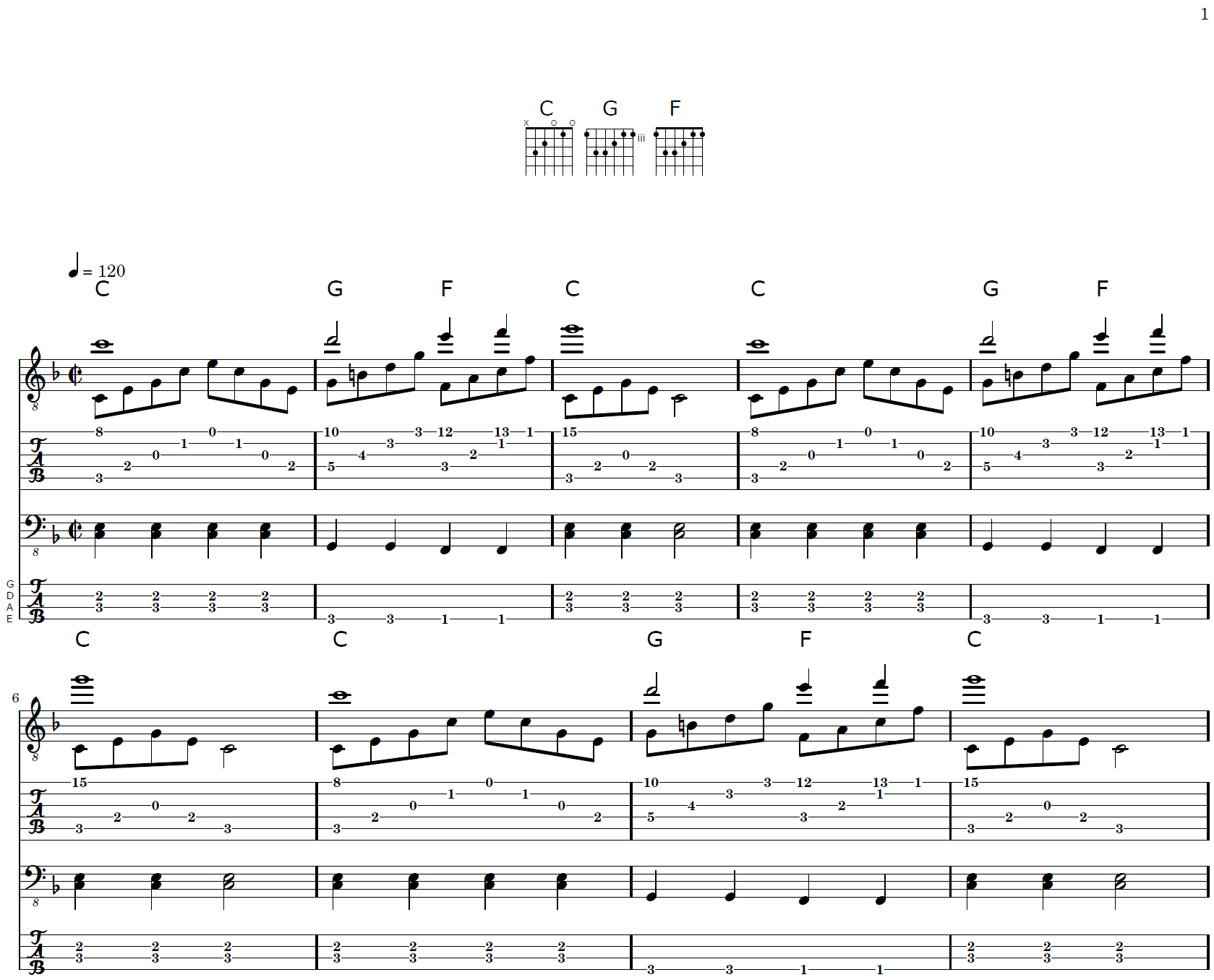
t_all remains unchanged from here forward. In the next examples, all that is needed is to alter the chords and chord_seq arguments to score. First, define these named vectors. The chord progression is C G F C. The C chords last over measures one and three. The F and G chords split the second measure, one half each.
You can define these chords however you like. They do not necessarily have to refer to the broken chords represented by the second voice of the guitar track in the output, though that would be common. Let’s say the chords in the chord chart refer generally to chords you can use to strum along, but this generic strumming is not actually shown in the tab as an explicit track because the pattern is meant to be whatever you want to make of it. Let the C chord be the open C chord, matching the melody in voice two, but the F and G chords refer to six string bar chords.
Remember that the order of the chords in chords is the order they appear in the chord chart. It is customary to show them in the order in which they first appear in a song, so C G F here, but this is certainly not a rule. The important part is that you have complete control over this. Also, because you repeated the who piece of music, you have to repeat the named chord sequence of integers similarly or the sequence chord symbols above the top staff will terminate prematurely.
#> c g f
#> "x;3;2;o;1;o;" "3;5;5;4;3;3;" "1;3;3;2;1;1;"
#> c g f c c g f c c g f c
#> 1 2 2 1 1 2 2 1 1 2 2 1
Now create a version that only adds a chord chart.

The chart in the example above matches the order in which you defined your chord positions. Next, remake the score adding only the chord symbol sequence over the top staff. Remove the chord chart.

Finally, combine both.

These examples demonstrate the level of control you have over this type of content, which you can elect to include or exclude depending on your preferences and how important or helpful the supplemental information is for a given song.
�����������������������������������������������������������������������������������������������������������������������������������������������������tabr/inst/doc/tabr-tunings.html���������������������������������������������������������������������0000644�0001762�0000144�00000412420�13503467507�016244� 0����������������������������������������������������������������������������������������������������ustar �ligges��������������������������users������������������������������������������������������������������������������������������������������������������������������������������������������������������������������������������������������������������
This section covers differently strung guitars and string instruments as well as non-standard tunings. Different tunings can be associated with individual music staves and are therefore specified when calling track.
Arbitrary tunings
More importantly, track tuning can also be expressed using explicit pitch for completely arbitrary tunings with any number of strings (tabr technically supports up to seven strings as a general rule). While the predefined set is convenient, it is not necessary to use and this is where the use of alternate tunings really shines.
Any of the explicit tunings shown in the tunings table can be supplied to track exactly as shown instead of using the given names, or any other explicit tuning. Tuning can be provided using tick or integer octave numbering style.
When providing a tuning, names are checked first against the IDs in tunings. If there is no match, it is assumed to be an explicit tuning already. Some additional checks are performed to catch common user errors in entering a tuning.
Tuning for a track defaults to standard tuning on a six string guitar. The following calls are equivalent and result in the same explicit tuning stored in each of the the track tables.
#> # A tibble: 1 x 6
#> phrase tuning voice staff ms_transpose ms_key
#> <list> <chr> <int> <chr> <int> <chr>
#> 1 <phrase> e, a, d g b e' 1 treble_8 0 NA
#> # A tibble: 1 x 6
#> phrase tuning voice staff ms_transpose ms_key
#> <list> <chr> <int> <chr> <int> <chr>
#> 1 <phrase> e, a, d g b e' 1 treble_8 0 NA
#> # A tibble: 1 x 6
#> phrase tuning voice staff ms_transpose ms_key
#> <list> <chr> <int> <chr> <int> <chr>
#> 1 <phrase> e, a, d g b e' 1 treble_8 0 NA
Number of strings
While tabr has a focus on guitar tablature, it does offer some built in support for string instruments more generally.
A convenient approach taken by tabr is that the number of strings an instrument has, and in turn the number of horizontal lines in a rendered tablature staff, is inferred directly from the explicit tuning.
Take the predefined bass tuning (standard bass tuning) or the explicit tuning it is converted to by track, which is e,, a,, d, g,. This is a tuning that specifies four strings. This is all tabr needs to know and pass along to LilyPond to yield a tablature staff with four staff lines as opposed to the standard six line staff used for typical guitar tabs.
The next example shows three different tablature staves: six string guitar in standard tuning, four string bass in standard tuning, and just for illustration, a one string instrument tuning to the fourth octave C note.
guitar <- tuplet("e, a, d g b e'", 4)
bass <- p("e,, a,, d, g,", 4)
one_string <- p("c' d' e' f'", 4)
tracks <- trackbind(track(guitar, music_staff = NA),
track(bass, "bass", music_staff = NA),
track(one_string, "c'", music_staff = NA))
tracks
#> # A tibble: 3 x 7
#> phrase tuning voice staff ms_transpose ms_key tabstaff
#> <list> <chr> <int> <chr> <int> <chr> <int>
#> 1 <phrase> e, a, d g b e' 1 NA 0 NA 1
#> 2 <phrase> e,, a,, d, g, 1 NA 0 NA 2
#> 3 <phrase> c' 1 NA 0 NA 3

Notice that for tunings other than standard guitar, the default is to show the note each string is tuned to at the start of the tablature staff. These can be turning off in score using string_names = FALSE. For example, when making a pure bass tab in standard tuning, you might opt to exclude this. There must still be some familiarity with the instrument of course. In the case of the made up one string instrument, no one would know which octave the open C belongs to, but the person with such an instrument would surely know what to expect.
Take another look at the same example, but this time including music staves. Because of the different octave ranges of the different instruments, it is best to use an appropriate clef. Recall the default (used for guitar) is treble_8 because guitar is a transposing instrument. Compare this with treble used for the third instrument that is in a higher octave. These different notations help prevent difficult to read transcriptions where the notes go far above or below the staff lines.
#> # A tibble: 3 x 7
#> phrase tuning voice staff ms_transpose ms_key tabstaff
#> <list> <chr> <int> <chr> <int> <chr> <int>
#> 1 <phrase> e, a, d g b e' 1 treble_8 0 NA 1
#> 2 <phrase> e,, a,, d, g, 1 bass_8 0 NA 2
#> 3 <phrase> c' 1 treble 0 NA 3

Current limitations
Although tabr infers the an instrument’s number of strings from its tuning, there are limitations. Chord fretboard diagrams are only supported for guitar, six string guitar specifically. If attempting to pass four or five strings of information to chord_set for bass, ukulele or banjo for example, this will incompletely fill in a six string guitar fretboard diagram in the chord chart of the output. Similarly, if attempting to provide seven strings for a seven string guitar, the chord chart will show the additional note, but it will be floating to the side of the chart. A seventh string line is not added to the diagram. Number of strings inferred from instrument tuning displays in the tablature staff, but does not generalize to fretboard diagrams.
������������������������������������������������������������������������������������������������������������������������������������������������������������������������������������������������������������������������������������������������tabr/inst/doc/tabr-phrases.html���������������������������������������������������������������������0000644�0001762�0000144�00001527364�13503467465�016244� 0����������������������������������������������������������������������������������������������������ustar �ligges��������������������������users������������������������������������������������������������������������������������������������������������������������������������������������������������������������������������������������������������������
Overview
This section goes into deeper detail on building musical phrases out of individual notes using the various component parts available for phrase construction. It also describes how to add information, note metadata, to the notes in a phrase so that the phrase is defined unambiguously.
As mentioned in the last section, phrases in tabr do not require a strict definition. It is recommended to keep phrases short enough that they do not cause you difficulty dissecting them again visually. They should also represent meaningful or at least convenient segments of music, for example whole measures, a particular rhythm section, or an identifiable section of a longer solo.
Writing out music in R code is not intended to be any more readable than writing out LilyPond markup. The driving motivation here is a preference for avoiding writing LilyPond markup directly, aimed at people who specifically want to do this from R. Care must still be taken to not write phrases that are so long and complex that even you can not adequately parse their information by eye afterward.
The opening section showed a basic example using a single, and very simple, phrase. This section will cover phrases that include notes and rests of different duration, slides, hammer ons and pull offs, simple string bends, and various other elements. Phrases will become longer and more visually complex. There is no way around this fact. But with proper care they can be kept manageable and interpretable, depending on your comfort level with music theory, notation and R programming.
Before diving in, take a look at the table to the right for an overview of some syntax and operators that are used throughout this section.
Notes
The first argument to phrase is notes. Notes are represented simply by the lowercase letters c d e f g a b.
Sharps and flats
Sharps are represented by appending # and flats with _, for example a# or b_. In phrases and the various tabr functions that operate on them, these two-character notes are tightly bound and treated as specific notes just like single letters.
Space-delimited time
A string of notes is separated in time by spaces. Simultaneous notes are not. For example, "a b c" represents a sequence of notes in time whereas "ceg" represents simultaneously played notes of a C major triad chord. For now the focus will remain on individual notes. The end of this section includes a tiny chord example. Chords are discussed in more detail in later sections.
Unambiguous pitch
While it is allowable to specify note sequences such as "a b c", this assumes octave number 3. But this may not be what you intend and there is no reason to assume anything. In the example here, what is likely intended might be "a2 b2 c3".
This is the recommended way to specify notes and requires this level of familiarity with describing musical pitch. LilyPond markup uses single or multiple consecutive commas for lower octaves and single quote marks for higher octaves. This notation is permitted by tabr as well. In fact, if you specify integer suffixes for octave numbering, phrase will reinterpret these for you. The following are equivalent, as shown when printing the LilyPond syntax generated by phrase.
The second example here also shows the convenient multiplicative expansion operator * that can be used inside character strings passed to the three main phrase arguments. Use this wherever convenient, though this tutorial section will continue to write things out explicitly for increased clarity. Other operators like this one to help shorten repetitive code are introduced later.
#> <Musical phrase>
#> <c,,>1 <c,>1 <c>1 <c'>1 <c''>1
#> <Musical phrase>
#> <c,,>1 <c,>1 <c>1 <c'>1 <c''>1
For more extreme octaves, the latter style requires more typing and is more difficult to read. However, some may find it easier to read for chords like an open E minor "e,b,egbe'" compared to either "e2b2e3g3b3e4" or "e2b2egbe4".
In tabr the two formats are referred to as integer and tick octave numbering. Note that octave number three corresponds to the central (no comma or single quote tick) octave with the tick numbering style. This is why 3 can be left out and not a number you might otherwise have suspected like 1 or 0. c3 corresponds to the lowest C note on a standard tuned guitar: fifth string, third fret. The lowest note in standard tuning on a six string guitar is the low open E, which is e2. Octave numbering begins from C: ...B2 C3 C#3...
Rests and ties
Rests and tied notes are actually part of the note argument. Both have duration, which is what belongs in info.
Rests are denoted by "r". In general, string specification is irrelevant for rests because nothing is played, so you can use a placeholder like x instead of a string number (see next section on string numbers). For the moment this example is not specifying the optional argument, string, so this can be ignored. Replacing some notes in the previous phrase with rests looks like the following.

At first glance, tied notes might seem like something that ought to be described via info. Even though the second note is not played, a tied note is still distinct from the note to which it is tied as far as notation is concerned.
For example, when tying a note over to a new measure, it must be included twice in notes. The tie is annotated on the original note with a ~ as follows.

The note is played once and has a duration of one and a quarter measures, but is still annotated as one quarter note tied to one whole note.
Explicit string-fret combinations
Specifying the exact pitch is still ambiguous for guitar tablature because the same note can be played in different positions along the neck of a guitar. Tabs show which string is fretted and where. For example, in standard tuning, the same C3 note can be played on the fifth string, third fret, or on the sixth string, eighth fret. If left unspecified, most guitar tablature software will attempt to guess where to play notes on the guitar. This is not done by some kind of impressive, reliable artificial intelligence. It usually just means arbitrarily reducing notes to the lowest possible frets even if a combination of notes would not make sense or be physically practical for someone to play them that way.
There is one degree of freedom when the note is locked in but its position is not. It is not necessary to specify both the string number and the fret number. Providing one implicitly locks in the other. If you know the pitch and the string number, the fret is known. LilyPond accepts string numbers readily. To isolate these numbers from the info argument notation in phrase, they are provided in the third argument, string, which is also helpful because string is always optional.
Returning to the earlier phrase, without the rests, the equivalent phrase with explicit string numbers would have had string = "5 4 4 4 3 3 2 2 2 2". The second version with rests could have been provided as string = "x 4 4 x 3 x 2 x 2 x". Instead, play further up the neck beginning with C3 on the sixth string, eighth fret.

Some programs like LilyPond allow for specifying a minimum fret threshold, such that every note is played at that fret or above. This would work better for some songs than others of course. It is still not as powerful or ideal as being explicit about every note’s position. This threshold option is not currently supported by tabr. It is recommended to always be explicit anyway, as it leads to more accurate guitar tablature. There is a preponderance of highly inaccurate guitar tabs in the online world. Please do not add to the heap.
Note metadata continued
This section returns to the info argument to phrase with more examples of various pieces of note information that can be bound to notes.
Dotted notes
Note duration was introduced earlier, but incompletely. Dotted notes can be used to add 50% more time to a note. For example, a dotted quarter note, given by "4.", is equal in length to a quarter note plus an eighth note, covering three eighths of a measure. Double dotted may also be supplied. "2.." represents one half note plus one quarter note plus another eight note duration, for a total of 4 + 2 + 1 = 7 eighths of a measure.
A couple measures with no rests that contains dotted and double dotted notes might look like this.
Dots are tightly bound in dotted notes. tabr treats these multi-character time durations as singular elements, just as it does for, say, sixteenth notes given by a "16".

Staccato
Notes played staccato are specified by appending a closing square bracket directly on the note duration, e.g., altering "16" to "16]". This will place a dot in the output below notes that are played staccato.

Muted or dead notes
Muted or dead notes are indicated by appending an "x" to a note duration, e.g., "8x".

Multiple pieces of information can be strung together for a single note. For example, combining a muted note with staccato can be given as "8x]". In this early version of tabr, do this with caution, as not all orderings of note information have been thoroughly tested yet. Duration always comes first though. Some pieces of information are not meant to go together either, such as a staccato note that must essentially be held rather than released, for the purpose of sliding to another note. Use human judgment. If you don’t ever see something in sheet music, it may not work in tabr either.
In this case, the example will work with "8x]" or "8]x". In fact, even accidentally leaving an extra staccato indicator in as "8]x]", which does undesirably alter the output of phrase, will still be parsed by LilyPond correctly. Nevertheless, stick closely to patterns shown in these examples if possible.
Slides
Slides are partially implemented. They work well in tabr when sliding from one note to another note. Slides to a note that do not begin from a previous note and slides from a note that do not terminate at subsequent note are not implemented. This is usually done with a bit of a hack in LilyPond by bending from or to a grace note and then making the grace note invisible. This hack or some another approach has not been ported to tabr.

As a brief aside, note the use of * above in the string argument to reduce typing. It is necessary to specify string here in order to ensure the notes are all on the fifth string in the output. Any space-delimited elements in phrase can take advantage of this terminal element notation for multiplicative expansion of an element. Terminal means that it must be appended to the end of whatever is being expanded; nothing can follow it. c*4 a*2 expands to c c c c a a inside phrase. 4.-*2 is replaced with 4.- 4.-. This convenient multiplicative expansion operator within character strings passed to phrase is available for the notes, info and string arguments.
Hammer ons and pull offs
Hammer ons and pull offs use the same notation and are essentially equivalent to slurs. They require a starting and stopping point. Therefore, they must always come in pairs. Providing an odd number of slur indicators will throw an error. The beginning of a slur is indicated using an open parenthesis, (, and the end of a slur is indicated with a closing parenthesis, ).
Editing the previous example, change some of the slides to hammer ons and pull offs.
- Change the opening two slides (C to B to C) to use a pull off followed by a hammer on. Note that each must be opened and closed, hence the
)( appended to the B, the second eighth note. Using only a single set of parentheses, opening on the first note and closing on the third, would make a single, general slur over all three in the output.
- Next, hammer on from D to E, pick E, and pull off back to D. Notice the notation is identical for in both directions. Whether the slur between the two consecutive notes is a hammer on or pull off is implicit, given by the direction.
- Then play the C-B-C part again, but differently from the opening. Pick, pick, hammer on, pick, and then the final slide.
- Finally, transpose up one octave by increasing the octave numbers attached to the pitches in
notes. The reason for this is simply to demonstrate the placement of slurs above or below notes on the tablature staff depending on the string number. With this transposition, move from the fifth to the third string.

Another brief aside: tabr has some helper functions that make your work a bit easier and your code a bit more legible, ideally both. Using meaningful separation helps keep the code relatively readable and easier to make changes to when you realize you made a mistake somewhere. Don’t write one enormous string representing an entire song. Aside from the avoiding code duplication where there is musical repetition, even something that might not repeat such as a guitar solo still benefits greatly from being broken up in to manageable parts.
glue is used above to combine both parts fed to notes rather than write a single character string. glue is a convenient function for joining strings in tabr. It’s a simple wrapper around paste that maintains space-delimitation as well as the phrase class when at least one element passed to glue is a phrase object. The string passed to info does not change between parts so it can be duplicated. Using the *n within-string operator from earlier does not apply here, but another function much like glue is dup. It is a wrapper around rep that is convenient in a tabr context. Like glue, it maintains the phrase class when applicable.
String bending
String bends are available but currently have a limited implementation in tabr and bend engraving in LilyPond itself is not fully developed. Specifying all kinds of bending, and doing so elegantly and yielding an aesthetically pleasing and accurate result, is immensely difficult. Bends are specified with a ^. Bend engraving does not look very good at the moment and control over how a bend is drawn and any associated notation indicating the number of semitones to bend is currently excluded.
In the example below, a half step bend-release-bend is attempted over the three B notes shown at the end of the first phrase. Because the string is only plucked one time, the first two B notes are tied through to the third. Since a tied note is a note, this is done in notes. The two bends are indicated with ^ on the first and third notes via info. A similar approach is taken with the second phrase, although with full step bends from G to A. In both cases, the initial bend is not a pre-bend, but should be very quick. None of these fine details can be provided with the current version of tabr.

As you can see, the implementation is limited in tabr. It is also relatively difficult to achieve natively in LilyPond. The bends are different but the number of steps must be inferred from the key. The timing of bends and releases is challenging. The engraving is poor. But it is a start point.
Chords
Chords are covered in detail in later sections. For now, a brief example is given to more fully demonstrate the concept of space-delimited time and the use of simultaneous vs. sequential notes in tabr. The example below shows how to include some open C major chords inside notes. It is simply a matter of removing spaces. The tightly bound notes are simultaneous in time. info applies to the entire chord because it describes attributes of notes played at a given moment. There are obvious limitations to this though fortunately not hugely detrimental. string numbers are tightly bound for chords as well.
It can be seen above that just like individual notes, chords can be specified using any combination of tick or integer octave numbering. They are equivalent. Tick style may be more readable for some. Leaving out the integer 3 can help for many chords. Note the shorthand string numbering, 5s, used for the second C chord. This is useful for bar chords. [n]s runs from n to 1.

This covers the detailed introduction to phrases. The next section will cover related helper functions, some of which have already been seen.
����������������������������������������������������������������������������������������������������������������������������������������������������������������������������������������������������������������������������������������������������������������������������tabr/inst/doc/tabr-tunings.Rmd����������������������������������������������������������������������0000644�0001762�0000144�00000014232�13472050642�016012� 0����������������������������������������������������������������������������������������������������ustar �ligges��������������������������users������������������������������������������������������������������������������������������������������������������������������������������������������������������������������������������������������������������---
title: "Strings and tunings"
output: rmarkdown::html_vignette
vignette: >
%\VignetteIndexEntry{Non-standard tuning}
%\VignetteEngine{knitr::rmarkdown}
%\VignetteEncoding{UTF-8}
---
```{r setup, include = FALSE}
options(crayon.enabled = TRUE)
sgr_wrap <- function(x, options){
paste0("