The `stSpecies` dataset is just a small table that pairs species named with representative thumbnail avatars, mostly pulled from the Memory Alpha website. There is nothing map-related here, but these are used in this [Stellar Cartography](https://leonawicz.github.io/rtrek/articles/sc.html) example. It is similar to the Leaflet example above, but a bit more interesting, with markers to click on and information displays. In the course of the above map-related examples, a few functions have also been introduced. `st_tiles` takes an `id` argument that is mapped to the available tile sets in `stTiles` and returns the relevant URL. `st_tiles_data` takes the same `id` argument and returns a simple example data frame containing ancillary data related to the available locations from `stGeo`. The result is always the same except that the grid cells for locations change with respect to the chosen tile set. Finally, `tile_coords` can be applied to one of these data frames to add `x` and `y` columns for a CRS that Leaflet will understand. ## Star Trek API To use the words of the developers, the [STAPI](http://stapi.co/) is *the first public Star Trek API, accessible via REST and SOAP. It's an open source project, that anyone can contribute to.* The API is highly functional. Please do not abuse the API with constant requests. Their pages suggest no more than one request per second, but I would suggest ten seconds between successive requests. The default anti-DDOS measures in `rtrek` limit requests to one per second. You can update this global `rtrek` setting with `options`, e.g. `options(rtrek_antiddos = 10)` for a minimum ten second wait between API calls to be an even better neighbor. `rtrek` will not permit faster requests. If set below one second, the option is ignored and a warning thrown when making any API call. ### STAPI entities There a many fields, or entities, available in the API. The available IDs can be found in this table: ```{r stapiEntities} stapiEntities ``` These ID values are passed to `stapi` to perform a search using the API. The other columns provide some information about the object returned from a search. All entity searches return tibble data frames. You can inspect or unnest the column names of each table returned from every available entity search so you can see beforehand what variables are associated with each entity. ### Accessing the API Using `stapi` should be thought of as a three part process: * Determine how many pages of results exist for a particular entity search. * Only after taking care to do the previous step, perform the search to return search results. * If satellite data is needed on a unique observation in the search results, call `stapi` one more time referencing the specific observation. To determine how many pages of results exist for a given search, set `page_count = TRUE`. The impact on the API will be equivalent to only searching a single page of results. One page contains metadata including the total number of pages. Nothing is returned in this "safe mode", but the total number of search results available is printed to the console. Searching movies only returns one page of results. However, there are a lot of characters in the Star Trek universe. Check the total pages available for character search. ```{r stapi_safe} stapi("character", page_count = TRUE) ``` And that is with 100 results per page! The default `page = 1` only returns the first page. `page` can be a vector, e.g. `page = 1:62`. Results from multi-page searches are automatically combined into a single, constant data frame output. For the second call to `stapi`, return only page two here, which contains the character, Q (currently, pending future character database updates that may shift the indexing). In case that does change and Q is not always near the top of page two of the search results, the example further below hard-codes his unique/universal ID. ```{r stapi_search} stapi("character", page = 2) ``` Character tables can be sparse. There are a lot of variables, many of which will contain missing data for rare, esoteric characters. Even for more popular characters about whom much more universe lore has been uncovered, it still takes dedicated nerds to enter all the data in a database. When a dataset contains a `uid` column, this can be used subsequently to extract a satellite dataset about that particular observation that was returned in the original search. First you used safe mode, then search mode, and now switch from search mode to extraction mode to obtain data about Q, specifically. All that is required to do this is pass Q's `uid` to `stapi` and call the function one last time. When `uid` is no longer `NULL`, `stapi` knows not to bother with a search and makes a different type of API call requesting information about the uniquely identified entry. ```{r stapi_extract} Q <- "CHMA0000025118" Q <- stapi("character", uid = Q) library(dplyr) Q$episodes %>% select(uid, title, stardateFrom, stardateTo) ``` The data returned on Q is actually a large list, including multiple data frames. For simplicity only a piece of it is shown above. ## Star Trek novel text mining This section will be continued in a future version of `rtrek`. For now what is available is a dataset `stBooks` that compliments the `stBooksWP` dataset seen earlier. `stBooks` has a similar number of metadata entries for Star Trek books and there is considerable overlap between the two datasets. However, there are also considerable differences in entries as well as formatting. This dataset represents metadata parsed, imperfectly but painstakingly thoroughly, from actual Star Trek books. Compared to `stBooksWP`, which represents a scraping of Wikipedia information on Star Trek books, `stBooks` contains several different fields, including more useful fields for analysts such as the number of words and chapters in a book. ```{r stBooks} stBooks ``` Obviously, licensed book content itself cannot be shared as data, so it is not possible to provide capability in `rtrek` to enable analysts to perform their own unique text mining analyses on Star Trek novel corpura. However, future versions of `rtrek` will include more summary datasets that will aim to represent more intersting variables. Just a couple examples could be the relative frequency of popular characters' names per book, or a senitment analysis, or any other set of interesting metrics that could be used to inform suggested reading lists of various tiles or books by particular authors with a favored style or focus. ��������������������������������������������������������������������������������������������������������������������������������������������������������������������������������������������������������������������������������������������������������������������������������������������������������������������������������������������������������������rtrek/README.md�������������������������������������������������������������������������������������0000644�0001762�0000144�00000013674�13303401746�012674� 0����������������������������������������������������������������������������������������������������ustar �ligges��������������������������users������������������������������������������������������������������������������������������������������������������������������������������������������������������������������������������������������������������ rtrek
 ==============================================================================================================================================================================================================================================================================================
[](https://cran.r-project.org/package=rtrek) [](https://cran.r-project.org/package=rtrek) [](http://www.rdocumentation.org/packages/rtrek) [](https://travis-ci.org/leonawicz/rtrek) [](https://ci.appveyor.com/project/leonawicz/rtrek) [](https://codecov.io/github/leonawicz/rtrek?branch=master) [](https://gitter.im/leonawicz/rtrek)
The `rtrek` package provides datasets related to the Star Trek fictional universe and functions to assist with the data. It interfaces with [Wikipedia](https://www.wikipedia.org/), [STAPI](http://stapi.co/), [Memory Alpha](http://memory-alpha.wikia.com/wiki/Portal:Main) and [Memory Beta](http://memory-beta.wikia.com/wiki/Main_Page) to retrieve data, metadata and other information relating to Star Trek. It also contains local sample datasets covering a variety of topics such as Star Trek universe species data, geopolitical data, and summary datasets resulting from text mining analyses of Star Trek novels. The package also provides functions for working with data from other Star Trek-related R data packages containing larger datasets not stored in `rtrek`.
*Note: This package is in beta (and not just the quadrant). Breaking changes may occur.*
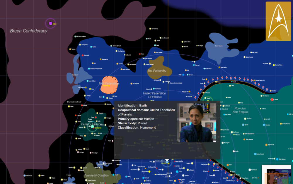
*Image: Example [Leaflet map](https://leonawicz.github.io/rtrek/articles/sc.html) using non-geographic Star Trek map tiles.*
==============================================================================================================================================================================================================================================================================================
[](https://cran.r-project.org/package=rtrek) [](https://cran.r-project.org/package=rtrek) [](http://www.rdocumentation.org/packages/rtrek) [](https://travis-ci.org/leonawicz/rtrek) [](https://ci.appveyor.com/project/leonawicz/rtrek) [](https://codecov.io/github/leonawicz/rtrek?branch=master) [](https://gitter.im/leonawicz/rtrek)
The `rtrek` package provides datasets related to the Star Trek fictional universe and functions to assist with the data. It interfaces with [Wikipedia](https://www.wikipedia.org/), [STAPI](http://stapi.co/), [Memory Alpha](http://memory-alpha.wikia.com/wiki/Portal:Main) and [Memory Beta](http://memory-beta.wikia.com/wiki/Main_Page) to retrieve data, metadata and other information relating to Star Trek. It also contains local sample datasets covering a variety of topics such as Star Trek universe species data, geopolitical data, and summary datasets resulting from text mining analyses of Star Trek novels. The package also provides functions for working with data from other Star Trek-related R data packages containing larger datasets not stored in `rtrek`.
*Note: This package is in beta (and not just the quadrant). Breaking changes may occur.*

*Image: Example [Leaflet map](https://leonawicz.github.io/rtrek/articles/sc.html) using non-geographic Star Trek map tiles.*
Installation ------------ Install the development version of `rtrek` from [GitHub](https://github.com/) with: ``` r # install.packages("devtools") devtools::install_github("leonawicz/rtrek") ``` Example -------
Use the Star Trek API (STAPI) to obtain information on the whereabouts and whenabouts of the infamous character, Q. Specifically, retrieve data on his appearances and the stardates when he shows up. The first API call does a lightweight, unobtrusive check to see how many pages of potential search results exist for characters in the database. There are a lot of characters. The second call grabs only page two results. The third call uses the universal/unique ID `uid` to retrieve data on Q. Think of these three successive uses of `stapi` as safe mode, search mode and extraction mode. ``` r library(rtrek) library(dplyr) stapi("character", page_count = TRUE) #> Total pages to retrieve all results: 62 stapi("character", page = 2) #> # A tibble: 100 x 24 #> uid name gender yearOfBirth monthOfBirth dayOfBirth placeOfBirth #>