The hardware and bandwidth for this mirror is donated by dogado GmbH, the Webhosting and Full Service-Cloud Provider. Check out our Wordpress Tutorial.
If you wish to report a bug, or if you are interested in having us mirror your free-software or open-source project, please feel free to contact us at mirror[@]dogado.de.
![]()
You can install:
The latest release version from CRAN with
install.packages("wbstats")or
The latest development version from github with
remotes::install_github("nset-ornl/wbstats")library(wbstats)
# Population for every country from 1960 until present
d <- wb_data("SP.POP.TOTL")
head(d)
#> # A tibble: 6 x 9
#> iso2c iso3c country date SP.POP.TOTL unit obs_status footnote last_updated
#> <chr> <chr> <chr> <dbl> <dbl> <chr> <chr> <chr> <date>
#> 1 AF AFG Afghanis~ 2019 38041754 <NA> <NA> <NA> 2020-07-01
#> 2 AF AFG Afghanis~ 2018 37172386 <NA> <NA> <NA> 2020-07-01
#> 3 AF AFG Afghanis~ 2017 36296400 <NA> <NA> <NA> 2020-07-01
#> 4 AF AFG Afghanis~ 2016 35383128 <NA> <NA> <NA> 2020-07-01
#> 5 AF AFG Afghanis~ 2015 34413603 <NA> <NA> <NA> 2020-07-01
#> 6 AF AFG Afghanis~ 2014 33370794 <NA> <NA> <NA> 2020-07-01wbstatslibrary(tidyverse)
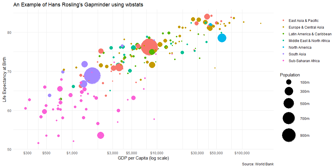
library(wbstats)
my_indicators <- c(
life_exp = "SP.DYN.LE00.IN",
gdp_capita ="NY.GDP.PCAP.CD",
pop = "SP.POP.TOTL"
)
d <- wb_data(my_indicators, start_date = 2016)
d %>%
left_join(wb_countries(), "iso3c") %>%
ggplot() +
geom_point(
aes(
x = gdp_capita,
y = life_exp,
size = pop,
color = region
)
) +
scale_x_continuous(
labels = scales::dollar_format(),
breaks = scales::log_breaks(n = 10)
) +
coord_trans(x = 'log10') +
scale_size_continuous(
labels = scales::number_format(scale = 1/1e6, suffix = "m"),
breaks = seq(1e8,1e9, 2e8),
range = c(1,20)
) +
theme_minimal() +
labs(
title = "An Example of Hans Rosling's Gapminder using wbstats",
x = "GDP per Capita (log scale)",
y = "Life Expectancy at Birth",
size = "Population",
color = NULL,
caption = "Source: World Bank"
) 
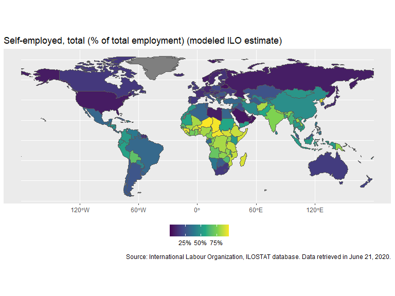
ggplot2 to
map wbstats datalibrary(rnaturalearth)
library(tidyverse)
library(wbstats)
ind <- "SL.EMP.SELF.ZS"
indicator_info <- filter(wb_cachelist$indicators, indicator_id == ind)
ne_countries(returnclass = "sf") %>%
left_join(
wb_data(
c(self_employed = ind),
mrnev = 1
),
c("iso_a3" = "iso3c")
) %>%
filter(iso_a3 != "ATA") %>% # remove Antarctica
ggplot(aes(fill = self_employed)) +
geom_sf() +
scale_fill_viridis_c(labels = scales::percent_format(scale = 1)) +
theme(legend.position="bottom") +
labs(
title = indicator_info$indicator,
fill = NULL,
caption = paste("Source:", indicator_info$source_org)
)
These binaries (installable software) and packages are in development.
They may not be fully stable and should be used with caution. We make no claims about them.
Health stats visible at Monitor.