The hardware and bandwidth for this mirror is donated by dogado GmbH, the Webhosting and Full Service-Cloud Provider. Check out our Wordpress Tutorial.
If you wish to report a bug, or if you are interested in having us mirror your free-software or open-source project, please feel free to contact us at mirror[@]dogado.de.
![]()
![]()
![]()
tidyvpc provides a flexible and comprehensive toolkit
for parameterizing a Visual Predictive Check (VPC) in R. With
tidyverse style syntax, you can chain together functions
(e.g., %>% or |>) to easily perform
stratification, censoring, prediction correction, and more.
tidyvpc supports both continuous and categorical VPC.
# CRAN
install.packages("tidyvpc")

# Development
# If there are errors (converted from warning) during installation related to packages
# built under different version of R, they can be ignored by setting the environment variable
# R_REMOTES_NO_ERRORS_FROM_WARNINGS="true" before calling remotes::install_github()

Sys.setenv(R_REMOTES_NO_ERRORS_FROM_WARNINGS="true")
remotes::install_github("certara/tidyvpc")tidyvpcThe Certara.VPCResults
package offers a Shiny app that can be used to easily generate the
underlying tidyvpc and ggplot2 code used to
create your VPC.
After importing the observed and simulated data into your R
environment, use the function vpcResultsUI()
to parameterize the VPC and customize the resulting plot output using
the Shiny GUI - then generate the R code to reproduce from command
line!
install.packages("Certara.VPCResults",
                 repos = c("https://certara.jfrog.io/artifactory/certara-cran-release-public/",
                           "https://cloud.r-project.org"),
                 method = "libcurl")

library(tidyvpc)
library(Certara.VPCResults)

vpcResultsUI(observed = obs_data[MDV == 0], simulated = sim_data[MDV == 0])
The Shiny application can serve as a learning heuristic and ensures
reproducibility by allowing you to save R and/or
Rmd scripts. Additionally, you may render RMarkdown to an
html, pdf, or docx output report.
Click here to
learn more about Certara.VPCResults.
tidyvpc requires a specific structure of observed and
simulated data in order to successfully generate VPC.
MDV == 0See tidyvpc::obs_data and tidyvpc::sim_data
for example data structures.
library(magrittr)
library(ggplot2)
library(tidyvpc)

# Filter MDV = 0
obs_data <- tidyvpc::obs_data[MDV == 0]
sim_data <- tidyvpc::sim_data[MDV == 0]

#Add LLOQ for each Study
obs_data$LLOQ <- obs_data[, ifelse(STUDY == "Study A", 50, 25)]

# Binning Method on x-variable (NTIME)
vpc <- observed(obs_data, x=TIME, y=DV) %>%
    simulated(sim_data, y=DV) %>%
    censoring(blq=(DV < LLOQ), lloq=LLOQ) %>%
    stratify(~ STUDY) %>%
    binning(bin = NTIME) %>%
    vpcstats()
Plot Code:
ggplot(vpc$stats, aes(x=xbin)) +
    facet_grid(~ STUDY) +
    geom_ribbon(aes(ymin=lo, ymax=hi, fill=qname, col=qname, group=qname), alpha=0.1, col=NA) +
    geom_line(aes(y=md, col=qname, group=qname)) +
    geom_line(aes(y=y, linetype=qname), size=1) +
    geom_hline(data=unique(obs_data[, .(STUDY, LLOQ)]),
        aes(yintercept=LLOQ), linetype="dotted", size=1) +
    geom_text(data=unique(obs_data[, .(STUDY, LLOQ)]),
        aes(x=10, y=LLOQ, label=paste("LLOQ", LLOQ, sep="="),), vjust=-1) +
    scale_colour_manual(
        name="Simulated Percentiles\nMedian (lines) 95% CI (areas)",
        breaks=c("q0.05", "q0.5", "q0.95"),
        values=c("red", "blue", "red"),
        labels=c("5%", "50%", "95%")) +
    scale_fill_manual(
        name="Simulated Percentiles\nMedian (lines) 95% CI (areas)",
        breaks=c("q0.05", "q0.5", "q0.95"),
        values=c("red", "blue", "red"),
        labels=c("5%", "50%", "95%")) +
    scale_linetype_manual(
        name="Observed Percentiles\n(black lines)",
        breaks=c("q0.05", "q0.5", "q0.95"),
        values=c("dotted", "solid", "dashed"),
        labels=c("5%", "50%", "95%")) +
    guides(
        fill=guide_legend(order=2),
        colour=guide_legend(order=2),
        linetype=guide_legend(order=1)) +
    theme(
        legend.position="top",
        legend.key.width=grid::unit(1, "cm")) +
    labs(x="Time (h)", y="Concentration (ng/mL)")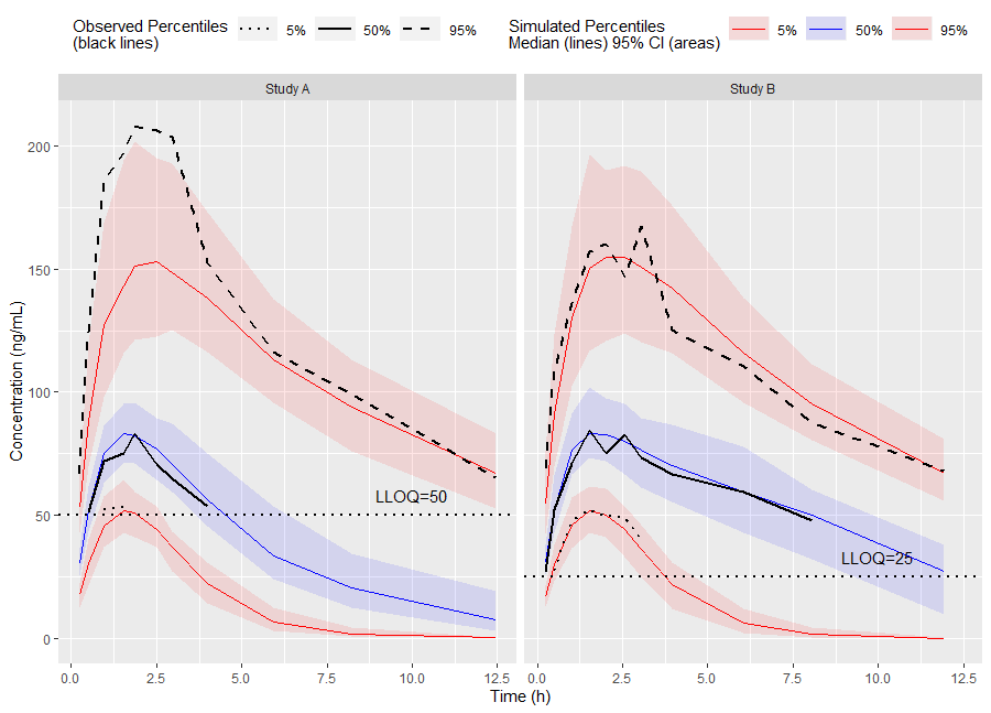
Or use the built-in plot() function from the
tidyvpc package.
# Binless method using 10%, 50%, 90% quantiles and LOESS Prediction Corrected

# Add PRED variable to observed data from first replicate of sim_data
obs_data$PRED <- sim_data[REP == 1, PRED]

vpc <- observed(obs_data, x=TIME, y=DV) %>%
    simulated(sim_data, y=DV) %>%
    stratify(~ GENDER) %>%
    predcorrect(pred=PRED) %>%
    binless(loess.ypc = TRUE) %>%
    vpcstats(qpred = c(0.1, 0.5, 0.9))

plot(vpc)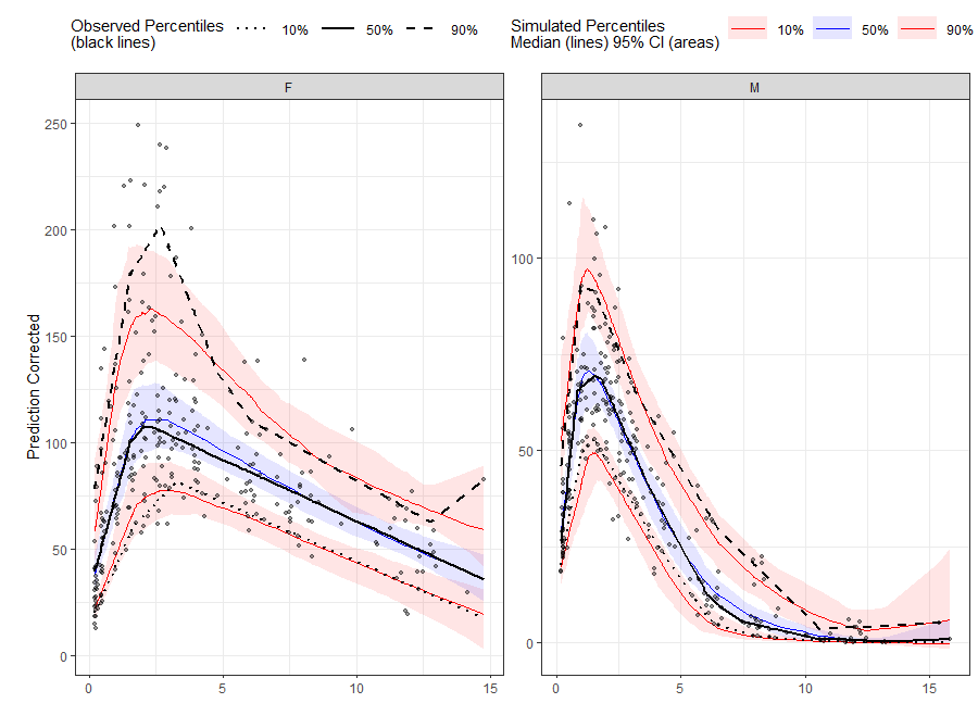
These binaries (installable software) and packages are in development.
They may not be fully stable and should be used with caution. We make no claims about them.
Health stats visible at Monitor.