The hardware and bandwidth for this mirror is donated by dogado GmbH, the Webhosting and Full Service-Cloud Provider. Check out our Wordpress Tutorial.
If you wish to report a bug, or if you are interested in having us mirror your free-software or open-source project, please feel free to contact us at mirror[@]dogado.de.
![]()
![]()
tabpfn, meaning prior fitted networks for tabular data, is a deep-learning model. See:
This R package is a wrapper of the Python library via reticulate. It has an idiomatic R syntax using standard S3 methods.
You can download the package from CRAN via:
install.packages("tabpfn")or you can install the development version of tabpfn like so:
require(pak)
pak(c("tidymodels/tabpfn"), ask = FALSE)
You’ll need a Python virtual environment to access the underlying library. After installing the R package, tabpfn will install the required Python bits when you first fit a model:
> library(tabpfn)
>
> predictors <- mtcars[, -1]
> outcome <- mtcars[, 1]
>
> # XY interface
> mod <- tab_pfn(predictors, outcome)
Downloading uv...Done!
Downloading cpython-3.12.12 (download) (15.9MiB)
 Downloading cpython-3.12.12 (download)
Downloading setuptools (1.1MiB)
Downloading scikit-learn (8.2MiB)
Downloading numpy (4.9MiB)

<downloading and installing more packages>

 Downloading llvmlite
 Downloading torch
Installed 58 packages in 350ms
> mod
tabpfn Regression Model

Training set
i 32 data points
i 10 predictorsAfter loading the package:
library(tabpfn)we can fit a model via the standard x/y interface.
set.seed(364)
reg_mod <- tab_pfn(mtcars[1:25, -1], mtcars$mpg[1:25])
reg_mod
#> TabPFN Regression Model
#> Training set
#> ℹ 25 data points
#> ℹ 10 predictors
There are also formula and recipes interfaces.
Prediction follows the usual S3 predict() method:
predict(reg_mod, mtcars[26:32, -1])
#> # A tibble: 7 × 1
#>   .pred
#>   <dbl>
#> 1  31.4
#> 2  24.3
#> 3  24.8
#> 4  16.4
#> 5  18.9
#> 6  14.4
#> 7  22.5
tabpfn follows the tidymodels prediction convention: a data frame is always returned with a standard set of column names.
For a classification model, the outcome should always be a factor vector. For example, using these data from the modeldata package:
library(modeldata)
#>
#> Attaching package: 'modeldata'
#> The following object is masked from 'package:datasets':
#>
#>     penguins
library(ggplot2)

two_cls_train <- parabolic[1:400,  ]
two_cls_val   <- parabolic[401:500,]
grid <- expand.grid(X1 = seq(-5.1, 5.0, length.out = 25),
                    X2 = seq(-5.5, 4.0, length.out = 25))

set.seed(3824)
cls_mod <- tab_pfn(class ~ ., data = two_cls_train)

grid_pred <- predict(cls_mod, grid)
grid_pred
#> # A tibble: 625 × 3
#>    .pred_Class1 .pred_Class2 .pred_class
#>           <dbl>        <dbl> <fct>
#>  1        0.997      0.00273 Class1
#>  2        0.998      0.00217 Class1
#>  3        0.998      0.00182 Class1
#>  4        0.998      0.00155 Class1
#>  5        0.998      0.00167 Class1
#>  6        0.998      0.00222 Class1
#>  7        0.996      0.00438 Class1
#>  8        0.989      0.0109  Class1
#>  9        0.948      0.0522  Class1
#> 10        0.745      0.255   Class1
#> # ℹ 615 more rows
The fit looks fairly good when shown with out-of-sample data:
cbind(grid, grid_pred) |>
  ggplot(aes(X1, X2)) +
  geom_point(
    data = two_cls_val,
    aes(col = class, pch = class),
    alpha = 3 / 4,
    cex = 3
  ) +
  geom_contour(
    aes(z = .pred_Class1),
    breaks = 1 / 2,
    col = "black",
    linewidth = 1
  ) +
  coord_equal(ratio = 1)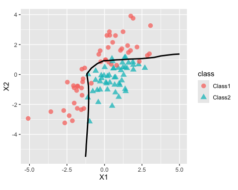
PriorLabs created the model. Starting with version 2.5, using TabPFN requires accepting the model license and setting a token. Each model version (v2.5, v2.6, etc.) has its own license that must be accepted individually.
To get access, visit https://ux.priorlabs.ai, go to the
Licenses tab (1), and accept the license for each model
version you intend to use (2). Then set the TABPFN_TOKEN
environment variable with the token from your account. Users who already
have TABPFN_TOKEN set can use TabPFN v2 without any
additional steps.

Also, the model is most effective when a GPU is available (by an order of magnitude or two). This may seem obvious to anyone already working with deep learning models, but it is a fairly new requirement for those strictly working with traditional tabular data models.
Please note that the tabpfn project is released with a Contributor Code of Conduct. By contributing to this project, you agree to abide by its terms.
These binaries (installable software) and packages are in development.
They may not be fully stable and should be used with caution. We make no claims about them.
Health stats visible at Monitor.