The hardware and bandwidth for this mirror is donated by dogado GmbH, the Webhosting and Full Service-Cloud Provider. Check out our Wordpress Tutorial.
If you wish to report a bug, or if you are interested in having us mirror your free-software or open-source project, please feel free to contact us at mirror[@]dogado.de.
The goal of stratifyR is to construct stratification boundaries using either the continuous variable in your data or a hypothetical distribution for your variable.
You can install stratifyR using:
install.packages("stratifyR")This is a basic example which shows you how to solve a common stratification problem:
library(stratifyR)
#> Loading required package: fitdistrplus
#> Loading required package: MASS
#> Loading required package: survival
#> Loading required package: zipfR
#> Loading required package: actuar
#>
#> Attaching package: 'actuar'
#> The following objects are masked from 'package:stats':
#>
#> sd, var
#> The following object is masked from 'package:grDevices':
#>
#> cm
#> Loading required package: triangle
#> Loading required package: mc2d
#> Loading required package: mvtnorm
#>
#> Attaching package: 'mc2d'
#> The following objects are masked from 'package:base':
#>
#> pmax, pmin
## basic example code using data
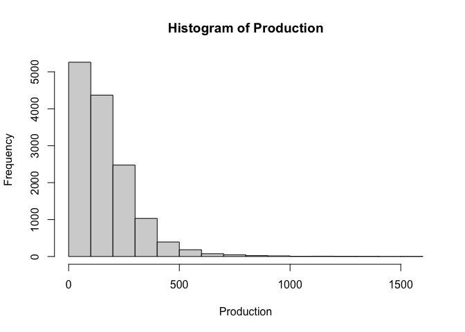
data(sugarcane)
Production <- sugarcane$Production
hist(Production)
res <- strata.data(Production, h = 2, n=1000)
#> The program is running, it'll take some time!
summary(res)
#> _____________________________________________
#> Optimum Strata Boundaries for h = 2
#> Data Range: [0.42, 1570.38] with d = 1569.96
#> Best-fit Frequency Distribution:  gamma
#> Parameter estimate(s):
#>       shape        rate
#> 1.520409984 0.009226811
#> ____________________________________________________
#>  Strata     OSB   Wh       Vh   WhSh   nh    Nh   fh
#>       1  195.18 0.68  2832.16 36.219  458  9456 0.05
#>       2 1570.38 0.32 18071.08 42.939  542  4438 0.12
#>   Total         1.00 20903.24 79.158 1000 13894 0.07
#> ____________________________________________________

## basic example code using distribution
res <- strata.distr(h=2, initval=0.65, dist=68, distr = "gamma",
params = c(shape=3.8, rate=0.55), n=500, N=10000)
#> The program is running, it'll take some time!
summary(res)
#> _____________________________________________
#> Optimum Strata Boundaries for h = 2
#> Data Range: [0.65, 68.65] with d = 68
#> Best-fit Frequency Distribution:  gamma
#> Parameter estimate(s):
#> shape  rate
#>  3.80  0.55
#> ____________________________________________________
#>  Strata   OSB   Wh    Vh  WhSh  nh    Nh   fh
#>       1  7.47 0.63  2.61 1.014 247  6279 0.04
#>       2 68.65 0.37  7.83 1.041 253  3721 0.07
#>   Total       1.00 10.44 2.055 500 10000 0.05
#> ____________________________________________________
The functions can be dynamically used to visualize the the strata boundaries, for 2 strata, over the density (or observations) of the “mag” variable from the quakes data (with purrr and ggplot2 packages loaded).
library(stratifyR)
library(ggplot2)
res <- strata.distr(h=2, initval=4, dist=2.4, distr = "lnorm",
params = c(meanlog=1.52681032, sdlog=0.08503554), n=300, N=1000)
#> The program is running, it'll take some time!
ggplot(data=quakes, aes(x = mag)) +
geom_density(fill = "blue", colour = "black", alpha = 0.3) +
geom_vline(xintercept = res$OSB, linetype = "dotted", color = "red")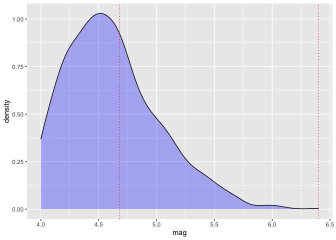 Read the
stratifyR vignette for a complete documentation and many more examples
using 10 different distributions.
Read the
stratifyR vignette for a complete documentation and many more examples
using 10 different distributions.
These binaries (installable software) and packages are in development.
They may not be fully stable and should be used with caution. We make no claims about them.
Health stats visible at Monitor.