The hardware and bandwidth for this mirror is donated by dogado GmbH, the Webhosting and Full Service-Cloud Provider. Check out our Wordpress Tutorial.
If you wish to report a bug, or if you are interested in having us mirror your free-software or open-source project, please feel free to contact us at mirror[@]dogado.de.
![]()
![]()
Supervised Variational Autoencoder (VAE) regression for high‑dimensional predictors (e.g., VIS–NIR–SWIR soil spectroscopy), implemented in Python TensorFlow/Keras and exposed in R via reticulate.
The README is also the main reproducible case study,
mirroring the vignette (vignettes/soilVAE-workflow.Rmd) so
a reader can understand the why, how, and
performance without opening additional files.
Given spectra \(x\in\mathbb{R}^p\) and a continuous soil property \(y\in\mathbb{R}\), soilVAE learns:
We minimize a weighted sum:
\[ \mathcal{L}(x,y) = \underbrace{\|x-\hat x\|_2^2}_{\text{reconstruction}} \;+\; \beta\;\underbrace{D_{KL}\!\left(q_\phi(z\mid x)\,\|\,\mathcal{N}(0,I)\right)}_{\text{regularization}} \;+\; \alpha\;\underbrace{\|y-\hat y\|_2^2}_{\text{regression}}. \]
In the package API, these correspond to beta_kl = β and
alpha_y = α.
install.packages("soilVAE")# install.packages("remotes")
remotes::install_github("HugoMachadoRodrigues/soilVAE")Because deep learning depends on external Python libraries, this README uses a defensive pattern:
Important:
reticulate“locks” the Python used per R session. If you change env variables oruse_*()calls, restart R.
library(reticulate)

# Make sure reticulate isn't forced to a missing python
Sys.unsetenv("RETICULATE_PYTHON")

# Create env (if needed)
if (!"soilvae-tf" %in% conda_list()$name) {
  conda_create("soilvae-tf", python_version = "3.11")
}

# Install core deps from conda-forge
conda_install("soilvae-tf", packages = c("pip", "numpy"), channel = "conda-forge")

# Install TF/Keras via pip inside the env
py_install(c("tensorflow>=2.13", "keras>=3"), pip = TRUE, envname = "soilvae-tf")
Now, in the same R session:
library(soilVAE)
soilVAE::vae_configure(conda = "soilvae-tf")
reticulate::py_config()library(soilVAE)
soilVAE::vae_configure(python = "C:/path/to/python.exe")This follows the workflow style commonly used in soil spectral inference tutorials (e.g., Wadoux et al., 2021) (Wadoux et al. 2021), with a direct comparison between a PLS baseline and soilVAE.
set.seed(19101991)

pkgs <- c("prospectr", "pls", "reticulate")
for (p in pkgs) if (!requireNamespace(p, quietly = TRUE)) install.packages(p)

library(prospectr)
library(pls)
library(reticulate)

if (!requireNamespace("soilVAE", quietly = TRUE)) {
  stop("soilVAE is not installed. Install it with remotes::install_github('HugoMachadoRodrigues/soilVAE').")
}
library(soilVAE)

# Defensive: detect Python + TF/Keras early, so the README can render everywhere.
has_py <- reticulate::py_available(initialize = FALSE)
has_tf <- FALSE
if (has_py) {
  try(reticulate::py_config(), silent = TRUE)
  has_tf <- reticulate::py_module_available("tensorflow") &&
    reticulate::py_module_available("keras")
}This example assumes you ship datsoilspc inside the
package (data/datsoilspc.rda).
This dataset is provided and described at Geeves et al. (1995)
Geeves, G. W. (Guy W.) & New South Wales. Department of Conservation and Land Management & CSIRO. Division of Soils. (1995). The physical, chemical and morphological properties of soils in the wheat-belt of southern N.S.W. and northern Victoria / G.W. Geeves … [et al.]. Glen Osmond, S. Aust. : CSIRO Division of Soils
data("datsoilspc", package = "soilVAE")
str(datsoilspc)
#> 'data.frame':    391 obs. of  5 variables:
#>  $ clay       : num  49 7 56 14 53 24 9 18 33 27 ...
#>  $ silt       : num  10 24 17 19 7 21 9 20 13 19 ...
#>  $ sand       : num  42 69 27 67 40 55 83 61 54 55 ...
#>  $ TotalCarbon: num  0.15 0.12 0.17 1.06 0.69 2.76 0.66 1.36 0.19 0.16 ...
#>  $ spc        : num [1:391, 1:2151] 0.0898 0.1677 0.0778 0.0958 0.0359 ...
#>   ..- attr(*, "dimnames")=List of 2
#>   .. ..$ : NULL
#>   .. ..$ : chr [1:2151] "350" "351" "352" "353" ...
#>  - attr(*, "na.action")= 'omit' Named int 392
#>   ..- attr(*, "names")= chr "63"
Expected structure:
datsoilspc$spc: matrix of reflectance spectra (rows =
samples; cols = wavelengths)datsoilspc$TotalCarbon: numeric target (example
property)We replicate typical “quantitative” metrics used in soil
spectroscopy:
RMSE, MAE, R², bias (ME), RPIQ, and RPD.
eval_quant <- function(y, yhat) {
  y <- as.numeric(y)
  yhat <- as.numeric(yhat)

  ok <- is.finite(y) & is.finite(yhat)
  y <- y[ok]
  yhat <- yhat[ok]

  if (length(y) < 3) {
    return(list(
      n = length(y),
      ME = NA_real_, MAE = NA_real_, RMSE = NA_real_,
      R2 = NA_real_, RPIQ = NA_real_, RPD = NA_real_
    ))
  }

  err <- yhat - y
  me <- mean(err)
  mae <- mean(abs(err))
  rmse <- sqrt(mean(err^2))

  ss_res <- sum((y - yhat)^2)
  ss_tot <- sum((y - mean(y))^2)
  r2 <- if (ss_tot == 0) NA_real_ else 1 - ss_res / ss_tot

  rpiq <- stats::IQR(y) / rmse
  rpd  <- stats::sd(y) / rmse

  list(
    n = length(y),
    ME = me,
    MAE = mae,
    RMSE = rmse,
    R2 = r2,
    RPIQ = rpiq,
    RPD = rpd
  )
}

as_df_metrics <- function(x) {
  data.frame(
    n = x$n,
    ME = round(x$ME, 2),
    MAE = round(x$MAE, 2),
    RMSE = round(x$RMSE, 2),
    R2 = round(x$R2, 2),
    RPIQ = round(x$RPIQ, 2),
    RPD = round(x$RPD, 2),
    stringsAsFactors = FALSE
  )
}matplot(
x = as.numeric(colnames(datsoilspc$spc)),
y = t(as.matrix(datsoilspc$spc)),
xlab = "Wavelength / nm",
ylab = "Reflectance",
ylim = c(0, 1),
type = "l",
lty = 1,
col = rgb(0.5, 0.5, 0.5, alpha = 0.3)
)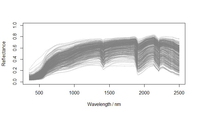
Raw reflectance spectra (datsoilspc$spc)
datsoilspc$spcA <- log(1 / as.matrix(datsoilspc$spc))

matplot(
  x = as.numeric(colnames(datsoilspc$spcA)),
  y = t(datsoilspc$spcA),
  xlab = "Wavelength / nm",
  ylab = "Absorbance",
  ylim = c(0, 4),
  type = "l",
  lty = 1,
  col = rgb(0.5, 0.5, 0.5, alpha = 0.3)
)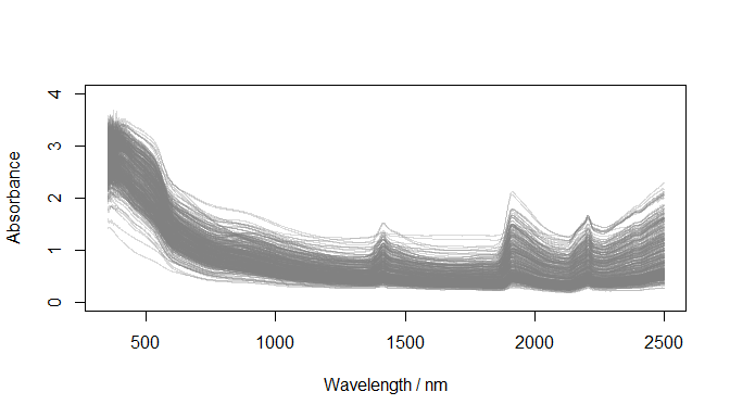
Absorbance spectra (datsoilspc$spcA)
oldWavs <- as.numeric(colnames(datsoilspc$spcA))
newWavs <- seq(min(oldWavs), max(oldWavs), by = 5)

datsoilspc$spcARs <- prospectr::resample(
  X = datsoilspc$spcA,
  wav = oldWavs,
  new.wav = newWavs,
  interpol = "linear"
)

datsoilspc$spcASnv <- prospectr::standardNormalVariate(datsoilspc$spcARs)
datsoilspc$spcAMovav <- prospectr::movav(datsoilspc$spcASnv, w = 11)

wavs <- as.numeric(colnames(datsoilspc$spcAMovav))

matplot(
  x = wavs,
  y = t(datsoilspc$spcAMovav),
  xlab = "Wavelength / nm",
  ylab = "Absorbance (SNV + movav)",
  type = "l",
  lty = 1,
  col = rgb(0.5, 0.5, 0.5, alpha = 0.3)
)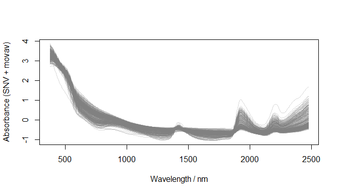
Preprocessed spectra (datsoilspc$spcAMovav)
set.seed(19101991)

calId <- sample(seq_len(nrow(datsoilspc)), size = round(0.75 * nrow(datsoilspc)))
datC <- datsoilspc[calId, ]
datV <- datsoilspc[-calId, ]  # <-- TEST

par(mfrow = c(1, 2))
hist(datC$TotalCarbon, main = "Calibration (datC)", xlab = "Total carbon")
hist(datV$TotalCarbon, main = "TEST (datV)", xlab = "Total carbon")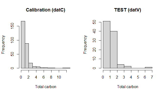
Calibration vs TEST splits (datC vs datV)
par(mfrow = c(1, 1))We fit PLS on calibration and evaluate on validation.
maxc <- 30

soilCPlsModel <- pls::plsr(
  TotalCarbon ~ spcAMovav,
  data = datC,
  method = "oscorespls",
  ncomp = maxc,
  validation = "CV"
)

plot(soilCPlsModel, "val", main = "PLS CV performance (datC)", xlab = "Number of components")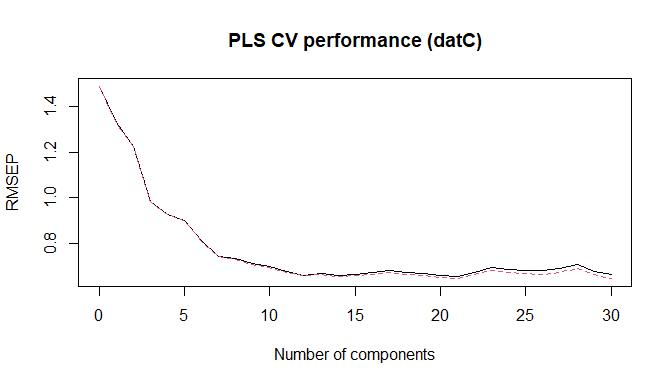
PLS CV performance (datC)
nc = 14).nc <- 14
# Refit on full datC with chosen nc (PLS itself uses all comps up to maxc; prediction uses nc)
soilCPlsPred_C <- as.numeric(predict(soilCPlsModel, ncomp = nc, newdata = datC$spcAMovav))
soilCPlsPred_T <- as.numeric(predict(soilCPlsModel, ncomp = nc, newdata = datV$spcAMovav))
par(mfrow = c(1, 2))
plot(datC$TotalCarbon, soilCPlsPred_C, xlab="Observed", ylab="Predicted", main="PLS (datC)", pch=16); abline(0,1)
plot(datV$TotalCarbon, soilCPlsPred_T, xlab="Observed", ylab="Predicted", main="PLS (TEST datV)", pch=16); abline(0,1)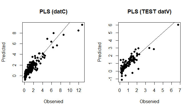
PLS predictions (datC + datV)
par(mfrow = c(1, 1))We use the same evaluation function used in many soilspec workflows.
pls_cal <- eval_quant(datC$TotalCarbon, soilCPlsPred_C)
pls_tst <- eval_quant(datV$TotalCarbon, soilCPlsPred_T)

as_df_metrics(pls_cal)
#>     n ME  MAE RMSE   R2 RPIQ  RPD
#> 1 293  0 0.37 0.56 0.86 2.04 2.63
as_df_metrics(pls_tst)
#>    n   ME  MAE RMSE   R2 RPIQ  RPD
#> 1 98 0.02 0.36 0.52 0.69 2.34 1.81This chunk detects if Python + TensorFlow + Keras can be
loaded.
If not available, the VAE section is skipped (vignette still
builds).
has_py <- reticulate::py_available(initialize = FALSE)

has_tf <- FALSE
if (has_py) {
  try(reticulate::py_config(), silent = TRUE)
  has_tf <- reticulate::py_module_available("tensorflow") &&
            reticulate::py_module_available("keras")
}

has_py
#> [1] TRUE
has_tf
#> [1] TRUE
Prepare Train/Val internal split within datC (no y transform; scale X only)
set.seed(19101991)

nC <- nrow(datC)
id_tr <- sample(seq_len(nC), size = round(0.80 * nC))
datC_tr <- datC[id_tr, ]
datC_va <- datC[-id_tr, ]

# y stays in original units (no transformation)
y_tr <- as.numeric(datC_tr$TotalCarbon)
y_va <- as.numeric(datC_va$TotalCarbon)

# X: scale predictors using TRAIN center/scale only
X_tr_raw <- as.matrix(datC_tr$spcAMovav)
X_va_raw <- as.matrix(datC_va$spcAMovav)
X_te_raw <- as.matrix(datV$spcAMovav)   # TEST

X_tr <- scale(X_tr_raw)
X_center <- attr(X_tr, "scaled:center")
X_scale  <- attr(X_tr, "scaled:scale")

# safe scaling: avoid division by zero
X_scale[X_scale == 0] <- 1

X_va <- scale(X_va_raw, center = X_center, scale = X_scale)
X_te <- scale(X_te_raw, center = X_center, scale = X_scale)

# sanity checks (dims)
dim(X_tr)
#> [1] 234 421
length(y_tr)
#> [1] 234
dim(X_va)
#> [1]  59 421
length(y_va)
#> [1] 59
dim(X_te)
#> [1]  98 421
Prepare Train/Val internal split within datC (no y transform; scale X only)
We model TotalCarbon using the preprocessed spectra
matrix spcAMovav.
reticulate::py_run_string("
import os
import random
import numpy as np
import tensorflow as tf

os.environ['PYTHONHASHSEED'] = '0'
random.seed(19101991)
np.random.seed(19101991)
tf.random.set_seed(19101991)
")

Sys.setenv(TF_DETERMINISTIC_OPS = "1")
Sys.setenv(TF_CPP_MIN_LOG_LEVEL = "2")         # reduce logs INFO/WARN
# Sys.setenv(TF_ENABLE_ONEDNN_OPTS = "0")

if (!has_tf) {
  message("TensorFlow/Keras not available; skipping soilVAE section.")
} else {

  Sys.setenv(TF_ENABLE_ONEDNN_OPTS="0")

  # Optional: force a specific python/venv/conda, if needed.
  # soilVAE::vae_configure(conda = "soilvae-tf")

  grid_vae <- data.frame(
    latent_dim = c(8L, 16L, 32L, 64L),
    dropout    = c(0.20, 0.30),
    lr         = c(5e-4),
    beta_kl    = c(0.01),
    alpha_y    = c(5),
    epochs     = c(500L),
    batch_size = c(64L, 128L),
    patience   = c(50L),
    stringsAsFactors = FALSE
  )

  grid_vae$hidden_enc <- list(c(512L, 256L, 128L))
  grid_vae$hidden_dec <- list(c(128L, 256L, 512L))

  tuned <- soilVAE::tune_vae_train_val(
    X_tr = X_tr, y_tr = y_tr,
    X_va = X_va, y_va = y_va,
    seed = 19101991,
    grid_vae = grid_vae
  )

  best <- soilVAE::select_best_from_grid(tuned$tuning_df, selection_metric = "euclid")

  cfg <- best$best

  # Refit on full datC (train+val) using early stopping monitored on the internal val (datC_va)
  m_vae <- soilVAE::vae_build(
    input_dim  = ncol(X_tr),
    hidden_enc = as.integer(strsplit(cfg$hidden_enc_str, "-")[[1]]),
    hidden_dec = as.integer(strsplit(cfg$hidden_dec_str, "-")[[1]]),
    latent_dim = as.integer(cfg$latent_dim),
    dropout    = as.numeric(cfg$dropout),
    lr         = as.numeric(cfg$lr),
    beta_kl    = as.numeric(cfg$beta_kl),
    alpha_y    = as.numeric(cfg$alpha_y)
  )

  soilVAE::vae_fit(
    model = m_vae,
    X = X_tr, y = y_tr,
    X_val = X_va, y_val = y_va,
    epochs = as.integer(cfg$epochs),
    batch_size = as.integer(cfg$batch_size),
    patience = as.integer(cfg$patience),
    verbose = 0L
  )

  yhat_tr <- as.numeric(soilVAE::vae_predict(m_vae, X_tr))
  yhat_va <- as.numeric(soilVAE::vae_predict(m_vae, X_va))
  yhat_te <- as.numeric(soilVAE::vae_predict(m_vae, X_te))

  # Metrics: internal train/val + FINAL TEST
  vae_trn <- eval_quant(y_tr, yhat_tr)
  vae_val <- eval_quant(y_va, yhat_va)
  vae_tst <- eval_quant(as.numeric(datV$TotalCarbon), yhat_te)

  # Plots
  par(mfrow = c(1, 3))
  plot(y_tr, yhat_tr, main="soilVAE (Train)", xlab="Observed", ylab="Predicted", pch=16); abline(0,1)
  plot(y_va, yhat_va, main="soilVAE (Val)",   xlab="Observed", ylab="Predicted", pch=16); abline(0,1)
  plot(as.numeric(datV$TotalCarbon), yhat_te, main="soilVAE (TEST datV)", xlab="Observed", ylab="Predicted", pch=16); abline(0,1)
  par(mfrow = c(1, 1))
}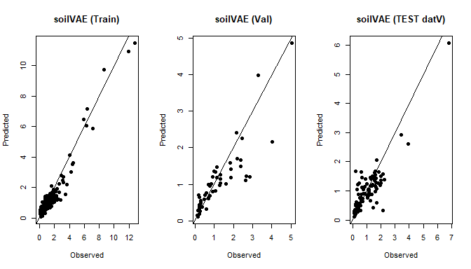
Train/Val splits for soilVAE
We present a compact comparison table.
if (!has_tf) {

  tab <- rbind(
    cbind(Model = "PLS", Split = "Calibration (datC)", as_df_metrics(pls_cal)),
    cbind(Model = "PLS", Split = "TEST (datV)",        as_df_metrics(pls_tst))
  )

} else {

  tab <- rbind(
    cbind(Model = "PLS",    Split = "Calibration (datC)", as_df_metrics(pls_cal)),
    cbind(Model = "PLS",    Split = "TEST (datV)",        as_df_metrics(pls_tst)),
    cbind(Model = "soilVAE",Split = "Train (internal)",   as_df_metrics(vae_trn)),
    cbind(Model = "soilVAE",Split = "Val (internal)",     as_df_metrics(vae_val)),
    cbind(Model = "soilVAE",Split = "TEST (datV)",        as_df_metrics(vae_tst))
  )

}

row.names(tab) <- NULL
tab
#>     Model              Split   n    ME  MAE RMSE   R2 RPIQ  RPD
#> 1     PLS Calibration (datC) 293  0.00 0.37 0.56 0.86 2.04 2.63
#> 2     PLS        TEST (datV)  98  0.02 0.36 0.52 0.69 2.34 1.81
#> 3 soilVAE   Train (internal) 234 -0.07 0.31 0.44 0.92 2.54 3.60
#> 4 soilVAE     Val (internal)  59 -0.10 0.33 0.51 0.76 2.36 2.04
#> 5 soilVAE        TEST (datV)  98 -0.04 0.33 0.47 0.74 2.56 1.97
If TensorFlow/Keras was not available, you can still use the PLS section and install a compatible Python stack later.
The PLS workflow depends only on R packages pls and
prospectr.
The supervised VAE requires:
-   Python (\>= 3.9)

-   TensorFlow (\>= 2.13)

- Keras (\>= 3)Education without ethics is only rhetoric.
Power without reflection is violence
These binaries (installable software) and packages are in development.
They may not be fully stable and should be used with caution. We make no claims about them.
Health stats visible at Monitor.