The hardware and bandwidth for this mirror is donated by dogado GmbH, the Webhosting and Full Service-Cloud Provider. Check out our Wordpress Tutorial.
If you wish to report a bug, or if you are interested in having us mirror your free-software or open-source project, please feel free to contact us at mirror[@]dogado.de.
![]()
rsgeo is an interface to the Rust libraries
geo-types and geo. geo-types
implements pure rust geometry primitives. The geo library
adds additional algorithm functionalities on top of
geo-types. This package lets you harness the speed, safety,
and memory efficiency of these libraries. geo-types does
not support Z or M dimensions. There is no support for CRS at this
moment.
# install.packages(
#   'rsgeo',
#   repos = c('https://josiahparry.r-universe.dev', 'https://cloud.r-project.org')
# )
library(rsgeo)
rsgeo works with vectors of geometries. When we compare this to
sf this is always the geometry column which is a class
sfc object (simple feature column).
# get geometry from sf
data(guerry, package = "sfdep")

polys <- guerry[["geometry"]] |>
  sf::st_cast("POLYGON")

# cast to rust geo-types
rs_polys <- as_rsgeo(polys)

head(rs_polys)
#> <rs_POLYGON[6]>
#> [1] Polygon { exterior: LineString([Coord { x: 801150.0, y: 2092615.0 }, Coord...
#> [2] Polygon { exterior: LineString([Coord { x: 729326.0, y: 2521619.0 }, Coord...
#> [3] Polygon { exterior: LineString([Coord { x: 710830.0, y: 2137350.0 }, Coord...
#> [4] Polygon { exterior: LineString([Coord { x: 882701.0, y: 1920024.0 }, Coord...
#> [5] Polygon { exterior: LineString([Coord { x: 886504.0, y: 1922890.0 }, Coord...
#> [6] Polygon { exterior: LineString([Coord { x: 747008.0, y: 1925789.0 }, Coord...
Cast geometries to sf
sf::st_as_sfc(rs_polys)
#> Geometry set for 116 features
#> Geometry type: POLYGON
#> Dimension:     XY
#> Bounding box:  xmin: 47680 ymin: 1703258 xmax: 1031401 ymax: 2677441
#> CRS:           NA
#> First 5 geometries:
#> POLYGON ((801150 2092615, 800669 2093190, 80068...
#> POLYGON ((729326 2521619, 729320 2521230, 72928...
#> POLYGON ((710830 2137350, 711746 2136617, 71243...
#> POLYGON ((882701 1920024, 882408 1920733, 88177...
#> POLYGON ((886504 1922890, 885733 1922978, 88547...
Calculate the unsigned area of polygons.
bench::mark(
  rust = unsigned_area(rs_polys),
  sf = sf::st_area(polys),
  check = FALSE
)
#> # A tibble: 2 × 6
#>   expression      min   median `itr/sec` mem_alloc `gc/sec`
#>   <bch:expr> <bch:tm> <bch:tm>     <dbl> <bch:byt>    <dbl>
#> 1 rust         55.6µs  57.65µs    16411.     3.8KB     0
#> 2 sf           1.36ms   1.44ms      649.   786.9KB     8.42
Find centroids
bench::mark(
  centroids(rs_polys),
  sf::st_centroid(polys),
  check = FALSE
)
#> # A tibble: 2 × 6
#>   expression                  min   median `itr/sec` mem_alloc `gc/sec`
#>   <bch:expr>             <bch:tm> <bch:tm>     <dbl> <bch:byt>    <dbl>
#> 1 centroids(rs_polys)    174.95µs    213µs     3720.     3.8KB     9.53
#> 2 sf::st_centroid(polys)   2.43ms    2.6ms      359.   892.9KB     4.70
Extract points coordinates
coords(rs_polys) |>
  head()
#>        x       y line_id polygon_id
#> 1 801150 2092615       1          1
#> 2 800669 2093190       1          1
#> 3 800688 2095430       1          1
#> 4 800780 2095795       1          1
#> 5 800589 2096112       1          1
#> 6 800333 2097190       1          1
Plot the polygons and their centroids
plot(rs_polys)
plot(centroids(rs_polys), add = TRUE)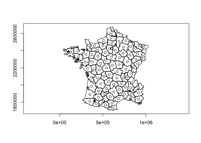
Calculate a distance matrix. Note that there is often floating point
error differences so check = FALSE in this case.
pnts <- centroids(rs_polys)
pnts_sf <- sf::st_as_sfc(pnts)

bench::mark(
  rust = distance_euclidean_matrix(pnts, pnts),
  sf = sf::st_distance(pnts_sf, pnts_sf),
  check = FALSE
)
#> # A tibble: 2 × 6
#>   expression      min   median `itr/sec` mem_alloc `gc/sec`
#>   <bch:expr> <bch:tm> <bch:tm>     <dbl> <bch:byt>    <dbl>
#> 1 rust       323.53µs 573.06µs     1540.     108KB     4.08
#> 2 sf           3.48ms   3.69ms      256.     351KB     0
Simplify geometries.
x <- rs_polys
x_simple <- simplify_geoms(x, 5000)

plot(x_simple)
bench::mark(
  rust = simplify_geoms(rs_polys, 500),
  sf = sf::st_simplify(polys, FALSE, 500),
  check = FALSE
)
#> # A tibble: 2 × 6
#>   expression      min   median `itr/sec` mem_alloc `gc/sec`
#>   <bch:expr> <bch:tm> <bch:tm>     <dbl> <bch:byt>    <dbl>
#> 1 rust         6.29ms   6.76ms      141.    1.91KB     0
#> 2 sf           8.52ms   9.02ms      108.    1.24MB     2.08
Union geometries with union_geoms(). Some things sf is
better at! One of which is performing unary unions of complex
geometries.
plot(union_geoms(rs_polys))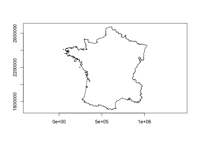
bench::mark(
  union_geoms(rs_polys),
  sf::st_union(polys),
  check = FALSE
)
#> # A tibble: 2 × 6
#>   expression                 min   median `itr/sec` mem_alloc `gc/sec`
#>   <bch:expr>            <bch:tm> <bch:tm>     <dbl> <bch:byt>    <dbl>
#> 1 union_geoms(rs_polys)    205ms    209ms      4.78        0B        0
#> 2 sf::st_union(polys)      120ms    134ms      7.49     921KB        0
We can cast between geometries as well.
lns <- cast_geoms(rs_polys, "linestring")Some unions are faster when using rsgeo vectors like linestrings.
lns_sf <- sf::st_cast(polys, "LINESTRING")

bench::mark(
  union_geoms(lns),
  sf::st_union(lns_sf),
  check = FALSE
)
#> # A tibble: 2 × 6
#>   expression                min   median `itr/sec` mem_alloc `gc/sec`
#>   <bch:expr>           <bch:tm> <bch:tm>     <dbl> <bch:byt>    <dbl>
#> 1 union_geoms(lns)      117.5µs    174µs    4275.         0B     0
#> 2 sf::st_union(lns_sf)   87.8ms     94ms      10.7    2.46MB     2.68
Find the closest point to a geometry
close_pnt <- closest_point(
  rs_polys,
  geom_point(800000, 2090000)
)

plot(rs_polys[1])
plot(close_pnt, pch = 15, add = TRUE)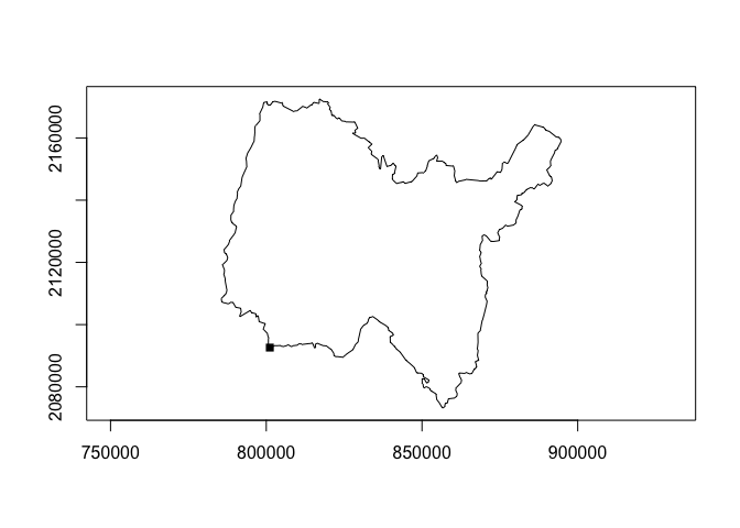
Find the haversine destination of a point, bearing, and distance. Compare to the very fast geosphere destination point function.
bench::mark(
  rust = haversine_destination(geom_point(10, 10), 45, 10000),
  Cpp = geosphere::destPoint(c(10, 10), 45, 10000),
  check = FALSE
)
#> # A tibble: 2 × 6
#>   expression      min   median `itr/sec` mem_alloc `gc/sec`
#>   <bch:expr> <bch:tm> <bch:tm>     <dbl> <bch:byt>    <dbl>
#> 1 rust         5.86µs   7.34µs   120442.     3.2KB     12.0
#> 2 Cpp         17.06µs  19.11µs    34150.    11.8MB     34.2
origin <- geom_point(10, 10)
destination <- haversine_destination(origin, 45, 10000)
plot(c(origin, destination), col = c("red", "blue"))
Find intermediate point on a great circle.
middle <- haversine_intermediate(origin, destination, 1/2)

plot(origin)
plot(destination, add = TRUE, col = "red")
plot(middle, add = TRUE, col = "blue")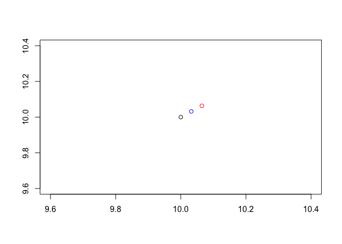
Find extreme coordinates with extreme_coords()
france <- union_geoms(rs_polys)

plot(france)
plot(extreme_coords(france)[[1]], add = TRUE, pch = 15)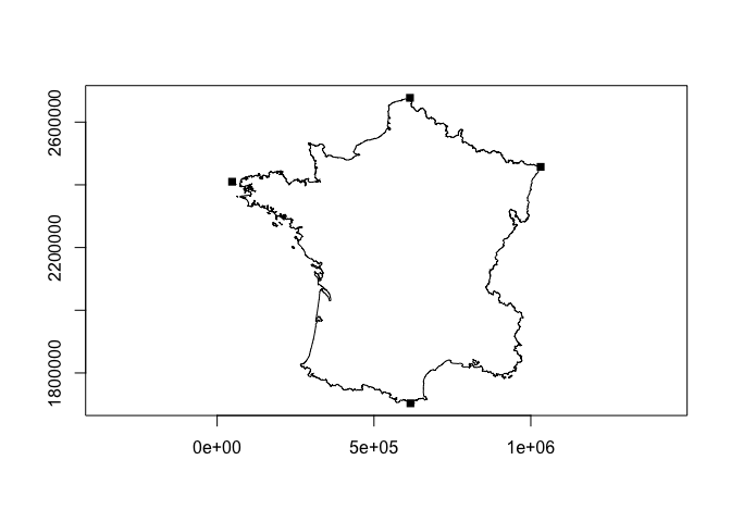
Get bounding rectangles
rects <- bounding_rect(rs_polys)
plot(rects)
Convex hulls
convex_hull(rs_polys) |>
  plot()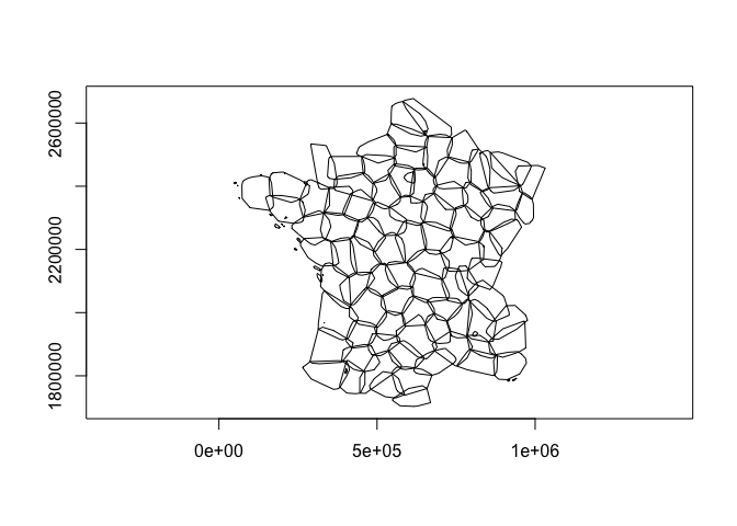
Expand into constituent geometries as a list of geometry vectors
expand_geoms(rs_polys) |>
  head()
#> [[1]]
#> <rs_LINESTRING[1]>
#> [1] LineString([Coord { x: 801150.0, y: 2092615.0 }, Coord { x: 800669.0, y: 2...
#>
#> [[2]]
#> <rs_LINESTRING[2]>
#> [1] LineString([Coord { x: 729326.0, y: 2521619.0 }, Coord { x: 729320.0, y: 2...
#> [2] LineString([Coord { x: 647667.0, y: 2468296.0 }, Coord { x: 647777.0, y: 2...
#>
#> [[3]]
#> <rs_LINESTRING[1]>
#> [1] LineString([Coord { x: 710830.0, y: 2137350.0 }, Coord { x: 711746.0, y: 2...
#>
#> [[4]]
#> <rs_LINESTRING[1]>
#> [1] LineString([Coord { x: 882701.0, y: 1920024.0 }, Coord { x: 882408.0, y: 1...
#>
#> [[5]]
#> <rs_LINESTRING[1]>
#> [1] LineString([Coord { x: 886504.0, y: 1922890.0 }, Coord { x: 885733.0, y: 1...
#>
#> [[6]]
#> <rs_LINESTRING[1]>
#> [1] LineString([Coord { x: 747008.0, y: 1925789.0 }, Coord { x: 746630.0, y: 1...
We can flatten the resultant geometries into a single vector using
flatten_geoms()
expand_geoms(rs_polys) |>
  flatten_geoms() |>
  head()
#> <rs_LINESTRING[6]>
#> [1] LineString([Coord { x: 801150.0, y: 2092615.0 }, Coord { x: 800669.0, y: 2...
#> [2] LineString([Coord { x: 729326.0, y: 2521619.0 }, Coord { x: 729320.0, y: 2...
#> [3] LineString([Coord { x: 647667.0, y: 2468296.0 }, Coord { x: 647777.0, y: 2...
#> [4] LineString([Coord { x: 710830.0, y: 2137350.0 }, Coord { x: 711746.0, y: 2...
#> [5] LineString([Coord { x: 882701.0, y: 1920024.0 }, Coord { x: 882408.0, y: 1...
#> [6] LineString([Coord { x: 886504.0, y: 1922890.0 }, Coord { x: 885733.0, y: 1...
Combine geometries into a single multi- geometry
combine_geoms(lns)
#> <rs_LINESTRING[1]>
#> [1] MultiLineString([LineString([Coord { x: 801150.0, y: 2092615.0 }, Coord { ...
Spatial predicates
x <- rs_polys[1:5]
intersects_sparse(x, rs_polys)
#> [[1]]
#> [1]  1 48 50 92 94
#>
#> [[2]]
#> [1]   2   7  63  78  80  81  98 101
#>
#> [[3]]
#> [1]  3 20 27 53 77 84 94
#>
#> [[4]]
#> [1]   4   5  30 107 109
#>
#> [[5]]
#> [1] 4 5 30 48Right now plotting is done using wk by first casting the
rsgeo into an sfc object.
These binaries (installable software) and packages are in development.
They may not be fully stable and should be used with caution. We make no claims about them.
Health stats visible at Monitor.