The hardware and bandwidth for this mirror is donated by dogado GmbH, the Webhosting and Full Service-Cloud Provider. Check out our Wordpress Tutorial.
If you wish to report a bug, or if you are interested in having us mirror your free-software or open-source project, please feel free to contact us at mirror[@]dogado.de.
Tools for binning data
![]()
![]()
# Install rbin from CRAN
install.packages("rbin")

# Or the development version from GitHub
# install.packages("devtools")
devtools::install_github("rsquaredacademy/rbin")rbin includes two addins for manually binning data:
rbinAddin()rbinFactorAddin()bins <- rbin_manual(mbank, y, age, c(29, 31, 34, 36, 39, 42, 46, 51, 56))
bins
#> Binning Summary
#> ---------------------------
#> Method Manual
#> Response y
#> Predictor age
#> Bins 10
#> Count 4521
#> Goods 517
#> Bads 4004
#> Entropy 0.5
#> Information Value 0.12
#>
#>
#> cut_point bin_count good bad woe iv entropy
#> 1 < 29 410 71 339 -0.483686036 2.547353e-02 0.6649069
#> 2 < 31 313 41 272 -0.154776266 1.760055e-03 0.5601482
#> 3 < 34 567 55 512 0.183985174 3.953685e-03 0.4594187
#> 4 < 36 396 45 351 0.007117468 4.425063e-06 0.5107878
#> 5 < 39 519 47 472 0.259825118 7.008270e-03 0.4383322
#> 6 < 42 431 33 398 0.442938178 1.575567e-02 0.3899626
#> 7 < 46 449 47 402 0.099298221 9.423907e-04 0.4836486
#> 8 < 51 521 40 481 0.439981550 1.881380e-02 0.3907140
#> 9 < 56 445 49 396 0.042587647 1.756117e-04 0.5002548
#> 10 >= 56 470 89 381 -0.592843261 4.564428e-02 0.7001343
# plot
plot(bins)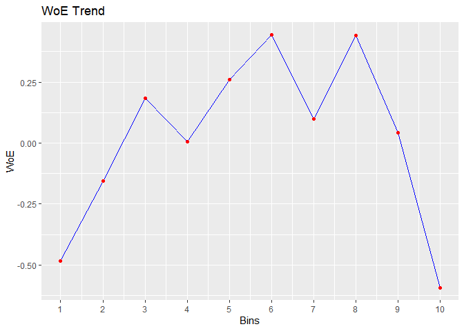
# combine levels
upper <- c("secondary", "tertiary")
out <- rbin_factor_combine(mbank, education, upper, "upper")
table(out$education)
#>
#>   upper unknown primary
#>    3651     179     691

# bins
bins <- rbin_factor(out, y, education)
bins
#> Binning Summary
#> ---------------------------
#> Method               Custom
#> Response             y
#> Predictor            education
#> Levels               3
#> Count                4521
#> Goods                517
#> Bads                 4004
#> Entropy              0.51
#> Information Value    0.01
#>
#>
#>     level bin_count good  bad         woe           iv   entropy
#> 1   upper      3651  426 3225 -0.02275738 0.0004219212 0.5197428
#> 2 primary       691   66  625  0.20109064 0.0057178780 0.4546110
#> 3 unknown       179   25  154 -0.22892949 0.0022651110 0.5833603

# plot
plot(bins)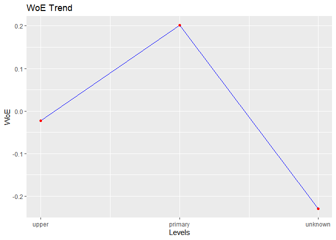
bins <- rbin_quantiles(mbank, y, age, 10)
bins
#> Binning Summary
#> -----------------------------
#> Method               Quantile
#> Response             y
#> Predictor            age
#> Bins                 10
#> Count                4521
#> Goods                517
#> Bads                 4004
#> Entropy              0.5
#> Information Value    0.12
#>
#>
#>    cut_point bin_count good bad          woe           iv   entropy
#> 1       < 29       410   71 339 -0.483686036 2.547353e-02 0.6649069
#> 2       < 31       313   41 272 -0.154776266 1.760055e-03 0.5601482
#> 3       < 34       567   55 512  0.183985174 3.953685e-03 0.4594187
#> 4       < 36       396   45 351  0.007117468 4.425063e-06 0.5107878
#> 5       < 39       519   47 472  0.259825118 7.008270e-03 0.4383322
#> 6       < 42       431   33 398  0.442938178 1.575567e-02 0.3899626
#> 7       < 46       449   47 402  0.099298221 9.423907e-04 0.4836486
#> 8       < 51       521   40 481  0.439981550 1.881380e-02 0.3907140
#> 9       < 56       445   49 396  0.042587647 1.756117e-04 0.5002548
#> 10     >= 56       470   89 381 -0.592843261 4.564428e-02 0.7001343

# plot
plot(bins)
bins <- rbin_winsorize(mbank, y, age, 10, winsor_rate = 0.05)
bins
#> Binning Summary
#> ------------------------------
#> Method               Winsorize
#> Response             y
#> Predictor            age
#> Bins                 10
#> Count                4521
#> Goods                517
#> Bads                 4004
#> Entropy              0.51
#> Information Value    0.1
#>
#>
#>    cut_point bin_count good bad        woe           iv   entropy
#> 1     < 30.2       723  112 611 -0.3504082 0.0224390979 0.6219926
#> 2     < 33.4       567   55 512  0.1839852 0.0039536848 0.4594187
#> 3     < 36.6       573   58 515  0.1367176 0.0022470488 0.4728562
#> 4     < 39.8       497   44 453  0.2846962 0.0079801719 0.4315480
#> 5       < 43       396   37 359  0.2253982 0.0040782670 0.4478305
#> 6     < 46.2       461   43 418  0.2272751 0.0048235624 0.4473095
#> 7     < 49.4       281   22 259  0.4187793 0.0092684760 0.3961315
#> 8     < 52.6       309   32 277  0.1112753 0.0008106706 0.4801796
#> 9     < 55.8       244   25 219  0.1231896 0.0007809490 0.4767424
#> 10   >= 55.8       470   89 381 -0.5928433 0.0456442813 0.7001343

# plot
plot(bins)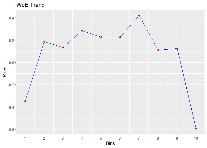
bins <- rbin_equal_length(mbank, y, age, 10)
bins
#> Binning Summary
#> ---------------------------------
#> Method               Equal Length
#> Response             y
#> Predictor            age
#> Bins                 10
#> Count                4521
#> Goods                517
#> Bads                 4004
#> Entropy              0.5
#> Information Value    0.17
#>
#>
#>    cut_point bin_count good  bad         woe           iv   entropy
#> 1     < 24.6        85   24   61 -1.11418623 0.0347480126 0.8586371
#> 2     < 31.2       822  106  716 -0.13676519 0.0035843196 0.5545619
#> 3     < 37.8      1133  115 1018  0.13365680 0.0042514380 0.4737339
#> 4     < 44.4       943   82  861  0.30436899 0.0171748162 0.4262287
#> 5       < 51       623   52  571  0.34913923 0.0146733167 0.4142794
#> 6     < 57.6       612   66  546  0.06595797 0.0005741022 0.4933757
#> 7     < 64.2       229   43  186 -0.58245971 0.0213871054 0.6967893
#> 8     < 70.8        34   12   22 -1.44087046 0.0255269312 0.9366674
#> 9     < 77.4        25   13   12 -2.12704897 0.0471100183 0.9988455
#> 10   >= 77.4        15    4   11 -1.03540535 0.0051663529 0.8366407

# plot
plot(bins)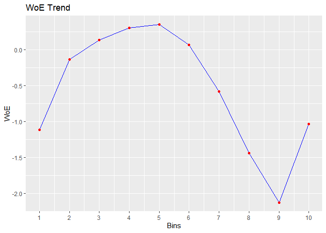
If you encounter a bug, please file a minimal reproducible example using reprex on github. For questions and clarifications, use StackOverflow.
Please note that the rbin project is released with a Contributor Code of Conduct. By contributing to this project, you agree to abide by its terms.
These binaries (installable software) and packages are in development.
They may not be fully stable and should be used with caution. We make no claims about them.
Health stats visible at Monitor.