The hardware and bandwidth for this mirror is donated by dogado GmbH, the Webhosting and Full Service-Cloud Provider. Check out our Wordpress Tutorial.
If you wish to report a bug, or if you are interested in having us mirror your free-software or open-source project, please feel free to contact us at mirror[@]dogado.de.

rbbnp

A Bias Bound Approach to Non-parametric Inference

This is an affiliated package for Susanne M Schennach, A Bias Bound Approach to Non-parametric Inference, The Review of Economic Studies, Volume 87, Issue 5, October 2020, Pages 2439–2472, https://doi.org/10.1093/restud/rdz065

version 0.1.0

Build up the package for your first time to use

Example: See the help documentation of a function

?biasBound_density

Load package

library(rbbnp)

Example Code

Loading Sample data

# Generate sample dataset
X = gen_sample_data(size = 1000, dgp = "2_fold_uniform", seed = 123456)
Y = -X^2 + 3*X + rnorm(1000)*X

For Stata/SAS/SPSS format dataset, one can use the haven package to load the dataset.

# Example for loading the Stata file
library(haven)
sample_data <- read_dta(file.path(EXT_DATA_PATH, "sample_data.dta"))
sample_data
# A tibble: 1,000 × 2
#        X     Y
#    <dbl> <dbl>
#  1 1.09  2.83 
#  2 1.63  2.01 
#  3 1.23  3.35 
#  4 1.07  1.95 
#  5 0.844 1.39 
#  6 0.879 1.95 
#  7 1.49  1.62 
#  8 0.699 2.04 
#  9 1.38  0.528
# 10 0.866 2.83 
# ℹ 990 more rows
# ℹ Use `print(n = ...)` to see more rows

1. Density estimation biasBound_density() function

If x is specified it will return the point estimation

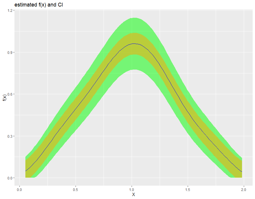
biasBound_density(X = X, x = 1, h = 0.09, alpha = 0.05, if_plot_ft = TRUE, kernel.fun = "Schennach2004")
# $est_Ar
# est_A    est_r 
# 4.297778 1.998942 
# 
# $b1x
# [1] 0.1270842
# 
# $ft_plot
# 
# $f1x
# [1] 0.9598753
# 
# $CI
# lb        ub 
# 0.7245948 1.1951559 

If not, it returns the estimation over the whole range of X

biasBound_density(X = X, h = 0.09, alpha = 0.05, if_plot_ft = TRUE, kernel.fun = "Schennach2004")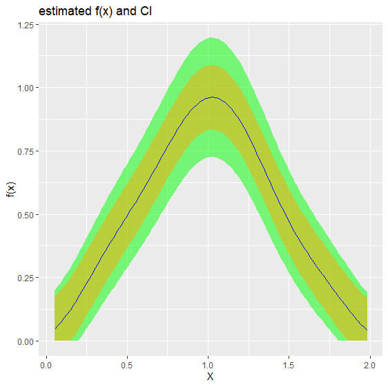

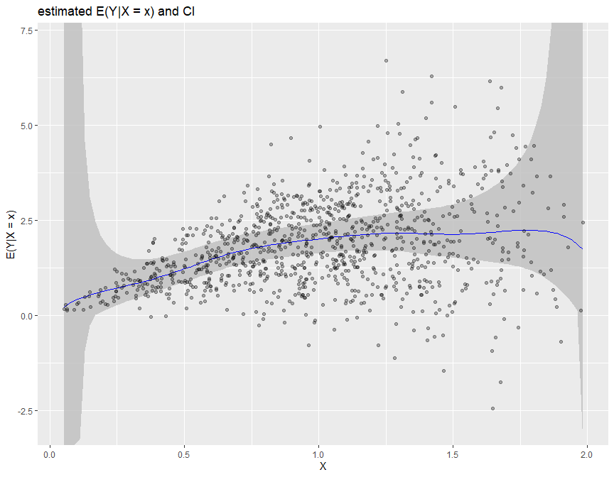
2. Conditional Mean estimation biasBound_condExpectation() function

If x is specified, it returns the point estimation of \(E(Y|X = x)\)

biasBound_condExpectation(Y = Y, X = X, x = 1, h = 0.09, alpha = 0.05, kernel.fun = "Schennach2004")

# $conditional_mean_yx
# [1] 2.001679
# 
# $CI
# lb       ub 
# 1.501453 2.609014 

If not, it returns the estimation over the whole range of X

biasBound_condExpectation(Y = Y, X = X, h = 0.09, alpha = 0.05, kernel.fun = "Schennach2004")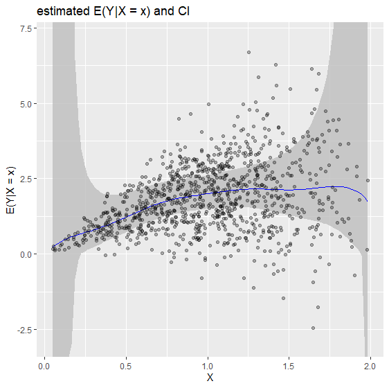

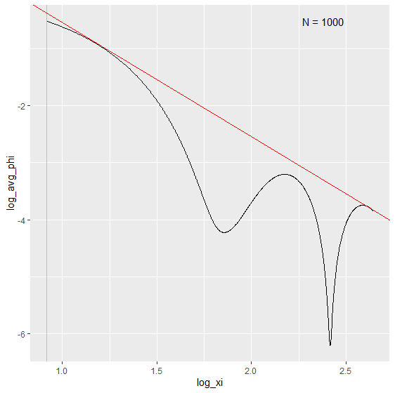
3. Fourier Transform frequency \(\xi\) interval selection

The Fourier Transform frequency \(\xi\) plays an important role in our bias bound approach. Specifically, it determines the range in which a nonparametric estimation the key parameters total variation \(A\) and order of differentiability \(r\) of the unknown distribution function. By default, it is determined by the Theorem 2 in Schennach (2020).

Here is an example how we can customize the range of \(\xi\) when performing the density and conditional expectation estimation.

# Example 1: Specifying x for point estimation with manually selected xi range from 1 to 12
biasBound_density(X = sample_data$X, x = 1, h = 0.09, xi_lb = 1, xi_ub = 12)
# $est_Ar
# est_A    est_r 
# 5.569499 2.229150 
# 
# $b1x
# [1] 0.07771575
# 
# $ft_plot

# Example 2: Density estimation with manually selected xi range from 1 to 12 xi_lb and xi_ub
biasBound_density(X = sample_data$X, h = 0.09, xi_lb = 1, xi_ub = 12, if_plot_ft = FALSE)

# Example 3: conditional expectation of Y on X with manually selected range of xi
biasBound_condExpectation(Y = sample_data$Y, X = sample_data$X, h = 0.09, xi_lb = 1, xi_ub = 12)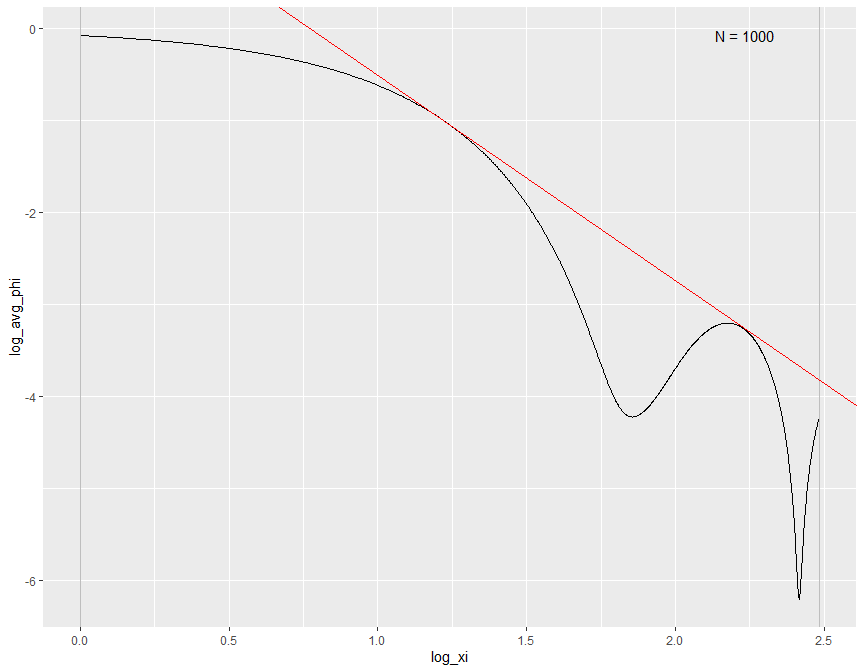

4. Kernel selection

We provide several options for kernel function, such as sinc, normal and epanechnikov kernel.

biasBound_density(X = sample_data$X, h = 0.09, methods_get_xi = "Schennach", if_plot_ft = TRUE, kernel.fun = "epanechnikov")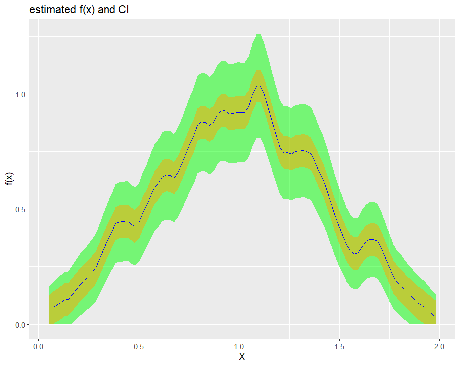

These binaries (installable software) and packages are in development.
They may not be fully stable and should be used with caution. We make no claims about them.
Health stats visible at Monitor.