The hardware and bandwidth for this mirror is donated by dogado GmbH, the Webhosting and Full Service-Cloud Provider. Check out our Wordpress Tutorial.
If you wish to report a bug, or if you are interested in having us mirror your free-software or open-source project, please feel free to contact us at mirror[@]dogado.de.

R package to simulate Probabilistic Long-Term Effects in models with temporal dependence

Christopher Gandrud and Laron K. Williams

Version: 1.0

About

pltesim implements Williams’s (2016) method for simulating probabilistic long-term effects in models with temporal dependence.

It is built on the coreSim package.

Process

To find and show probabilistic long-term effects in models with temporal dependence with pltesim:

1. Estimate the coefficients. Currently pltesim works with binary outcome models, e.g. logit, so use glm from the default R installation.

2. Create a data frame with your counterfactual. This should have a row with the fitted counterfactual values and columns with names matching those in your fitted model. All variables without values will be treated as 0 in the counterfactual.

3. Simulate the long-term effects with plte_builder.

4. Plot the results with plte_plot.

Examples

These examples replicate Figure 1 in Williams (2016). First estimate your model. You may need to use btscs to generate spells for the binary dependent variable.

library(pltesim)
library(ggplot2)

data('negative_year')

# BTSCS set the data
neg_set <- btscs(df = negative_year, event = 'y', t_var = 'year',
                 cs_unit = 'group', pad_ts = FALSE)

# Estimate the model
m1 <- glm(y ~ x + spell_time + I(spell_time^2) + I(spell_time^3),
          family = binomial(link = 'logit'),
          data = neg_set)

Then fit the counterfactual:

counterfactual <- data.frame(x = 0.5)

Now simulate and plot long-term effects for a variety of scenarios using plte_builder and plte_plot. plte_builder takes as its input the fitted model object with the estimated coefficients (obj), an identification of the basic time period variable (obj_tvar), the counterfactual (cf), how long the counterfactual persists (cf_duration, it is permanent by default), and the time period points over which to simulate the effects.

Note that by default the predicted probabilities from logistic regression models are found. You can specify a custom quantity of interest function with the FUN argument.

In this first example the counterfactual is persistent throughout the entire time span:

# Permanent
sim1 <- plte_builder(obj = m1, obj_tvar = 'spell_time',
                     cf = counterfactual, t_points = c(13, 25))

plte_plot(sim1) + ggtitle('Permanent')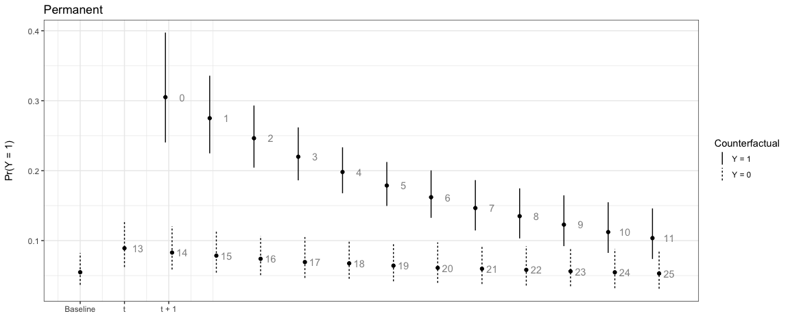

Note that the numbers next to each simulation point indicate the time since the last event. You can choose to not show these numbers by setting t_labels = FALSE in the plte_plot call.

In the next example, the effect only lasts for one time period:

# One-time
sim2 <- plte_builder(obj = m1, obj_tvar = 'spell_time', cf_duration = 'one-time',
                     cf = counterfactual, t_points = c(13, 25))

plte_plot(sim2) + ggtitle('One-time')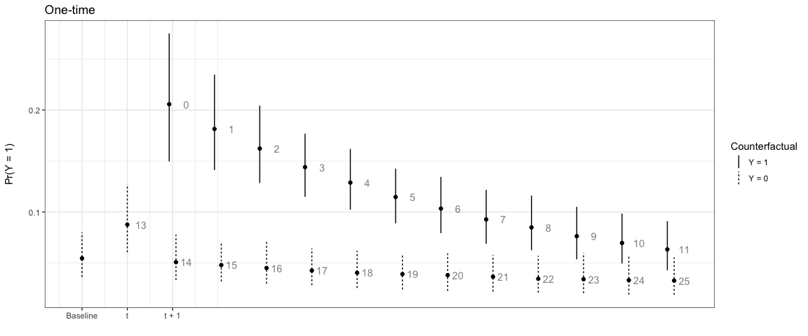

We can also have the counterfactual effect last for short periods of time and simulate the effect if another event occurs:

# Temporary
sim3 <- plte_builder(obj = m1, obj_tvar = 'spell_time', cf_duration = 4,
                     cf = counterfactual, t_points = c(13, 25))

plte_plot(sim3) + ggtitle('Temporary')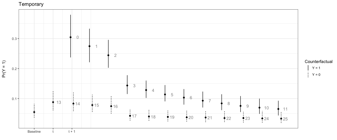

# Multiple events, permanent counter factual
sim4 <- plte_builder(obj = m1, obj_tvar = 'spell_time',
                     cf = counterfactual, t_points = c(13, 20, 25))

plte_plot(sim4) + ggtitle('Permanent, Multiple Events')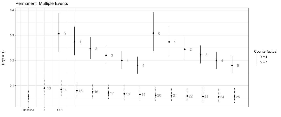

By default the baseline scenario has all covariate values fitted at 0. You can supply a custom baseline scenario in the second row of the counterfactual (cf) data frame. For example:

# Custom baseline scenario
counterfactual_baseline <- data.frame(x = c(1, 0.5))

sim5 <- plte_builder(obj = m1, obj_tvar = 'spell_time', cf_duration = 4,
                     cf = counterfactual_baseline, t_points = c(13, 25))

plte_plot(sim5) + ggtitle('Temporary, Custom Baseline')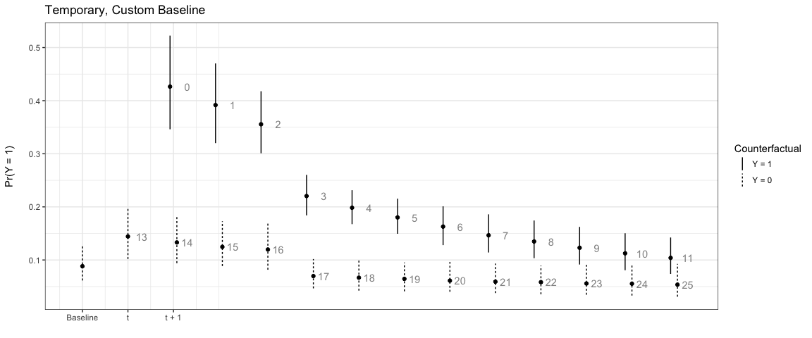

These binaries (installable software) and packages are in development.
They may not be fully stable and should be used with caution. We make no claims about them.
Health stats visible at Monitor.