

The hardware and bandwidth for this mirror is donated by dogado GmbH, the Webhosting and Full Service-Cloud Provider. Check out our Wordpress Tutorial.
If you wish to report a bug, or if you are interested in having us mirror your free-software or open-source project, please feel free to contact us at mirror[@]dogado.de.
mritc classifies the voxels of a structural brain
magnetic resonance image into cerebrospinal fluid (CSF), gray matter
(GM) and white matter (WM), using normal mixture models and hidden
Markov normal mixture models. Several fitting methods are provided, from
a plain EM algorithm through to Markov-chain Monte Carlo approaches that
also address the partial volume effect (where a voxel contains a mixture
of tissue types) and intensity non-uniformity (smoothly varying bias in
the scanner signal). The methods are described in Feng & Tierney
(2011).
You can install mritc from CRAN with
install.packages("mritc")or the development version from GitHub with
# install.packages("remotes")
remotes::install_github("jonclayden/mritc")The package includes a sample T1-weighted structural image and a corresponding brain mask, which we can use to demonstrate tissue classification.
library(mritc)

t1 <- readMRI(system.file("extdata", "t1.rawb.gz", package="mritc"),
              dim=c(91,109,91), format="rawb.gz")
mask <- readMRI(system.file("extdata", "mask.rawb.gz", package="mritc"),
                 dim=c(91,109,91), format="rawb.gz")

tc <- mritc(t1, mask, method="ICM", verbose=FALSE)
tc
## Using method ICM, among 237067 voxels,
## 18% are classified to CSF,
## 45% are classified to GM,
## 37% are classified to WM.
In this case the images are stored in a simple binary format,
requiring the dimensions to be specified, but readMRI() can
also handle NIfTI or ANALYZE files, or numeric arrays read by other
packages can be passed in.
The mritc() function is an interface to the various
classification methods available within the package, selected with its
“method” argument. The mask limits classification to within the
brain.
The summary() method gives a little more detail on the
fitted intensity distribution for each tissue type:
summary(tc)
## Using method ICM, the results are:
##     proportion%   mean standard deviation
## CSF          18  48.02              13.34
## GM           45  94.35              10.48
## WM           37 128.31              10.32
The plot() method shows the classified image, overlaid
with the tissue label at each voxel (0 = outside the brain mask, 1 =
CSF, 2 = GM, 3 = WM). By default since package version 0.6.0, this uses
the viewer from the
RNifti package; previously misc3d::slices3d()
was used, and this remains an option, although it requires system
support for Tk.
plot(tc, interactive=FALSE)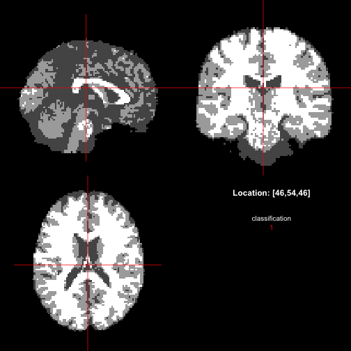
The package also bundles the “true” partial volume fractions for this
image, which can be compared to the fitted probabilities using
measureMRI(). This reports the mean squared error,
misclassification rate, relative volume error and Dice similarity for
each tissue type, and a confusion table.
csf <- readMRI(system.file("extdata", "csf.rawb.gz", package="mritc"),
               dim=c(91,109,91), format="rawb.gz")
gm <- readMRI(system.file("extdata", "gm.rawb.gz", package="mritc"),
              dim=c(91,109,91), format="rawb.gz")
wm <- readMRI(system.file("extdata", "wm.rawb.gz", package="mritc"),
              dim=c(91,109,91), format="rawb.gz")
truth <- cbind(csf[mask==1], gm[mask==1], wm[mask==1]) / 255

measureMRI(actual=truth, pre=tc$prob)
## $mse
## [1] 0.03309548
##
## $misclass
## [1] 0.09494362
##
## $rseVolume
## [1] 0.04655948 0.03611199 0.02440557
##
## $DSM
## [1] 0.9139096 0.8968206 0.9111253
##
## $conTable
##              [,1]       [,2]       [,3]
## [1,] 0.9351851852 0.04197286 0.00000000
## [2,] 0.0639774141 0.88062756 0.07775644
## [3,] 0.0008374007 0.07739958 0.92224356
See ?mritc for the other fitting methods available, and
?mritc-package for more background on the underlying
models.
These binaries (installable software) and packages are in development.
They may not be fully stable and should be used with caution. We make no claims about them.
Health stats visible at Monitor.