The hardware and bandwidth for this mirror is donated by dogado GmbH, the Webhosting and Full Service-Cloud Provider. Check out our Wordpress Tutorial.
If you wish to report a bug, or if you are interested in having us mirror your free-software or open-source project, please feel free to contact us at mirror[@]dogado.de.
![]()
This package is intended to help data scientists and decision-makers understand the potential value of churn prediction models depending on how many customers are being targeted by a campaign.
You can install the development version from GitHub with:
# install.packages("devtools")
devtools::install_github("PeerChristensen/modelimpact")The first three functions aim to provide information about the
business impact of using a model and targeting x % of the customer base.
These functions accept the following arguments (required ones in
bold):
x - a data frame fixed_cost - fixed costs (defaults to 0) var_cost - variable costs (defaults to 0) tp_val - true positive value (defaults to 0) prob_col - the variable containing
target class probabilitiestruth_col the variable containing the
actual classprofit_thresholds() accepts the following arguments:
x - a data frame var_cost - variable costs prob_accept - Probability of offer being accepted.
Defaults to 1. tp_val - The average value of a True Positive.
var_cost is automatically subtracted. fp_val - The average cost of a False Positive.
var_cost is automatically subtracted. tn_val - The average cost of a True Negatives fn_val - The average cost of a False Negatives
prob_col - The column with
probabilities of the event of interest truth_col - the column with the actual
outcome/class. Possible values are ‘Yes’ and ‘No’# Parameter settings
fixed_cost <- 1000
var_cost <- 100
tp_val <- 2000library(modelimpact)
library(tidyverse)
library(scales)
head(predictions)
#> # A tibble: 6 x 4
#> predict No Yes Churn
#> <chr> <dbl> <dbl> <chr>
#> 1 No 0.996 0.00353 No
#> 2 No 0.983 0.0166 No
#> 3 No 0.993 0.00705 No
#> 4 No 0.981 0.0187 No
#> 5 No 0.894 0.106 No
#> 6 No 0.997 0.00254 Nocost_rev <- predictions %>%
cost_revenue(
fixed_cost = fixed_cost,
var_cost = var_cost,
tp_val = tp_val,
prob_col = Yes,
truth_col = Churn)
head(cost_rev)
#> # A tibble: 6 x 4
#> row pct cost_sum cum_rev
#> <int> <int> <dbl> <dbl>
#> 1 1 1 1100 2000
#> 2 2 1 1200 4000
#> 3 3 1 1300 6000
#> 4 4 1 1400 6000
#> 5 5 1 1500 6000
#> 6 6 1 1600 8000# functions for formatting plotting axes
ks <- function (x) { number_format(accuracy = 1,
scale = 1/1000,
suffix = "k",
big.mark = ",")(x) }
pcts <- function (x) { percent_format(scale=1)((x / max(x)) * 100) }
theme_set(theme_minimal())
cost_rev %>%
ggplot() +
geom_line(aes(row,cost_sum), colour ="black",linetype="dashed") +
geom_line(aes(row,cum_rev), colour = "darkred",size=1) +
scale_y_continuous(labels = ks) +
scale_x_continuous(labels = pcts) +
labs(x = "% targeted",y = "Costs & revenue")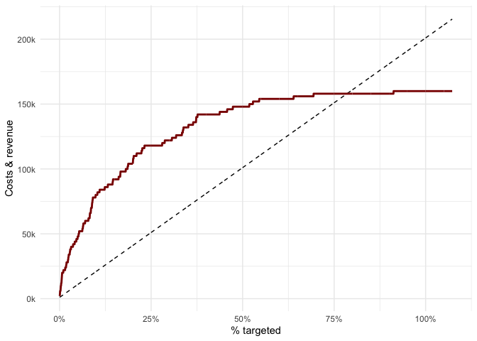
profit_df <- predictions %>%
  profit(
    fixed_cost = fixed_cost,
    var_cost   = var_cost,
    tp_val     = tp_val,
    prob_col   = Yes,
    truth_col  = Churn)

head(profit_df)
#> # A tibble: 6 x 3
#>     row   pct profit
#>   <int> <int>  <dbl>
#> 1     1     1    900
#> 2     2     1   2800
#> 3     3     1   4700
#> 4     4     1   4600
#> 5     5     1   4500
#> 6     6     1   6400
# max profit
max_profit <- profit_df %>% filter(profit == max(profit)) %>% select(row,pct,profit)
max_profit
#> # A tibble: 1 x 3
#> row pct profit
#> <int> <int> <dbl>
#> 1 464 22 70600profit_df %>%
ggplot(aes(x=row,y=profit)) +
geom_line(colour = "darkred",size=1) +
scale_y_continuous(labels = ks) +
geom_segment(x = max_profit$row, y= 0,xend=max_profit$row,
yend = max_profit$profit, colour="black",linetype="dashed") +
geom_hline(yintercept = 0,colour="black", linetype="dashed") +
scale_x_continuous(labels = pcts) +
labs(x = "% targeted",y = "Profit")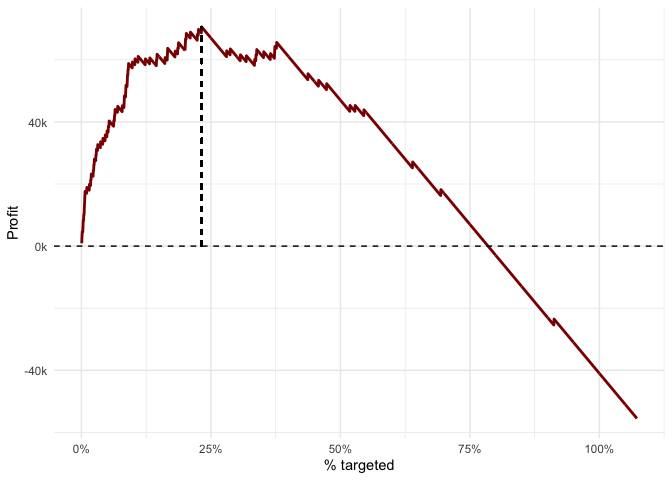
roi_df <- predictions %>%
  roi(
    fixed_cost = fixed_cost,
    var_cost   = var_cost,
    tp_val     = tp_val,
    prob_col   = Yes,
    truth_col  = Churn)

head(roi_df)
#> # A tibble: 6 x 5
#>     row   pct cum_rev cost_sum   roi
#>   <int> <int>   <dbl>    <dbl> <dbl>
#> 1     1     1    2000     1100 0.818
#> 2     2     1    4000     1200 2.33
#> 3     3     1    6000     1300 3.62
#> 4     4     1    6000     1400 3.29
#> 5     5     1    6000     1500 3
#> 6     6     1    8000     1600 4
roi_df %>%
ggplot(aes(x=row,y=roi)) +
geom_hline(yintercept = 0,colour="black", linetype="dashed") +
geom_line(colour = "darkred",size=1) +
scale_x_continuous(labels = pcts) +
labs(x = "% targeted",y = "ROI")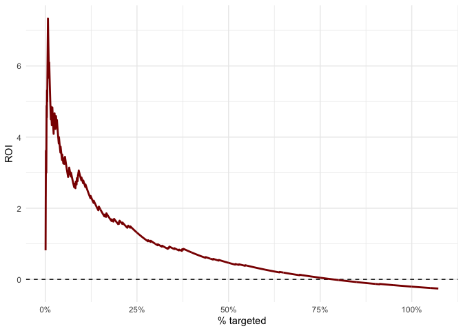
thresholds <- predictions %>%
  profit_thresholds(var_cost    = 100,
                    prob_accept = .7,
                    tp_val      = 2000,
                    fp_val      = 0,
                    tn_val      = 0,
                    fn_val      = -2000,
                    prob_col = Yes,
                    truth_col = Churn)

head(thresholds)
#> # A tibble: 6 x 2
#>   threshold payoff
#>       <dbl>  <dbl>
#> 1      0      9850
#> 2      0.01  68400
#> 3      0.02  67500
#> 4      0.03  42700
#> 5      0.04  42960
#> 6      0.05  20840
optimal_threshold <- thresholds %>% filter(payoff == max(payoff))
optimal_threshold
#> # A tibble: 1 x 2
#> threshold payoff
#> <dbl> <dbl>
#> 1 0.01 68400thresholds %>%
ggplot(aes(x=threshold,y=payoff)) +
geom_line(color="darkred",size = 1) +
geom_hline(yintercept=0,linetype="dashed") +
scale_y_continuous(labels = ks)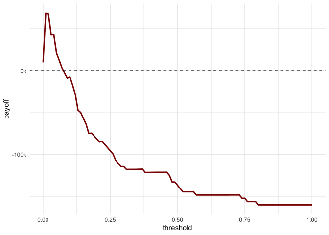
These binaries (installable software) and packages are in development.
They may not be fully stable and should be used with caution. We make no claims about them.
Health stats visible at Monitor.