The hardware and bandwidth for this mirror is donated by dogado GmbH, the Webhosting and Full Service-Cloud Provider. Check out our Wordpress Tutorial.
If you wish to report a bug, or if you are interested in having us mirror your free-software or open-source project, please feel free to contact us at mirror[@]dogado.de.
![]()
![]()
lvmisc is a package with miscellaneous R functions,
including basic data computation/manipulation, easy plotting and tools
for working with statistical models objects. You can learn more about
the methods for working with models in
vignette("working_with_models").
You can install the released version of lvmisc from CRAN with:
install.packages("lvmisc")And the development version from GitHub with:
# install.packages("devtools")
devtools::install_github("verasls/lvmisc")Some of what you can do with lvmisc.
library(lvmisc)
library(dplyr)

# Compute body mass index (BMI) and categorize it
starwars %>%
  select(name, birth_year, mass, height) %>%
  mutate(
    BMI = bmi(mass, height / 100),
    BMI_category = bmi_cat(BMI)
  )
#> # A tibble: 87 × 6
#>    name               birth_year  mass height   BMI BMI_category
#>    <chr>                   <dbl> <dbl>  <int> <dbl> <fct>
#>  1 Luke Skywalker           19      77    172  26.0 Overweight
#>  2 C-3PO                   112      75    167  26.9 Overweight
#>  3 R2-D2                    33      32     96  34.7 Obesity class I
#>  4 Darth Vader              41.9   136    202  33.3 Obesity class I
#>  5 Leia Organa              19      49    150  21.8 Normal weight
#>  6 Owen Lars                52     120    178  37.9 Obesity class II
#>  7 Beru Whitesun lars       47      75    165  27.5 Overweight
#>  8 R5-D4                    NA      32     97  34.0 Obesity class I
#>  9 Biggs Darklighter        24      84    183  25.1 Overweight
#> 10 Obi-Wan Kenobi           57      77    182  23.2 Normal weight
#> # … with 77 more rows

# Divide numerical variables in quantiles
divide_by_quantile(mtcars$wt, 4)
#>  [1] 2 2 1 2 3 3 3 2 2 3 3 4 4 4 4 4 4 1 1 1 1 3 3 4 4 1 1 1 2 2 3 2
#> Levels: 1 2 3 4

# Center and scale variables by group
center_variable(iris$Petal.Width, by = iris$Species, scale = TRUE)
#>   [1] -0.046 -0.046 -0.046 -0.046 -0.046  0.154  0.054 -0.046 -0.046 -0.146
#>  [11] -0.046 -0.046 -0.146 -0.146 -0.046  0.154  0.154  0.054  0.054  0.054
#>  [21] -0.046  0.154 -0.046  0.254 -0.046 -0.046  0.154 -0.046 -0.046 -0.046
#>  [31] -0.046  0.154 -0.146 -0.046 -0.046 -0.046 -0.046 -0.146 -0.046 -0.046
#>  [41]  0.054  0.054 -0.046  0.354  0.154  0.054 -0.046 -0.046 -0.046 -0.046
#>  [51]  0.074  0.174  0.174 -0.026  0.174 -0.026  0.274 -0.326 -0.026  0.074
#>  [61] -0.326  0.174 -0.326  0.074 -0.026  0.074  0.174 -0.326  0.174 -0.226
#>  [71]  0.474 -0.026  0.174 -0.126 -0.026  0.074  0.074  0.374  0.174 -0.326
#>  [81] -0.226 -0.326 -0.126  0.274  0.174  0.274  0.174 -0.026 -0.026 -0.026
#>  [91] -0.126  0.074 -0.126 -0.326 -0.026 -0.126 -0.026 -0.026 -0.226 -0.026
#> [101]  0.474 -0.126  0.074 -0.226  0.174  0.074 -0.326 -0.226 -0.226  0.474
#> [111] -0.026 -0.126  0.074 -0.026  0.374  0.274 -0.226  0.174  0.274 -0.526
#> [121]  0.274 -0.026 -0.026 -0.226  0.074 -0.226 -0.226 -0.226  0.074 -0.426
#> [131] -0.126 -0.026  0.174 -0.526 -0.626  0.274  0.374 -0.226 -0.226  0.074
#> [141]  0.374  0.274 -0.126  0.274  0.474  0.274 -0.126 -0.026  0.274 -0.226

# Quick and easy plotting with {ggplot}
plot_scatter(mtcars, disp, mpg, color = factor(cyl))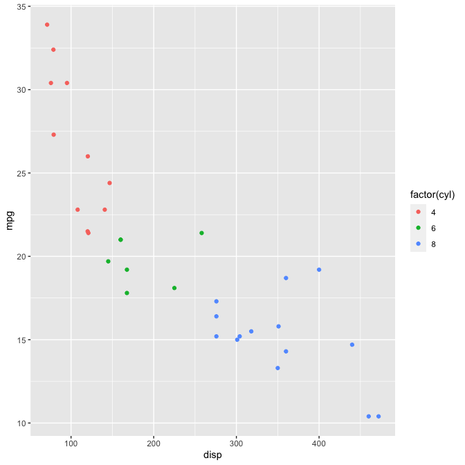
# Work with statistical model objects
m <- lm(disp ~ mpg + hp + cyl + mpg:cyl, mtcars)
accuracy(m)
#>      AIC    BIC   R2 R2_adj  MAE   MAPE  RMSE
#> 1 344.64 353.43 0.87   0.85 34.9 15.73% 43.75
plot_model(m)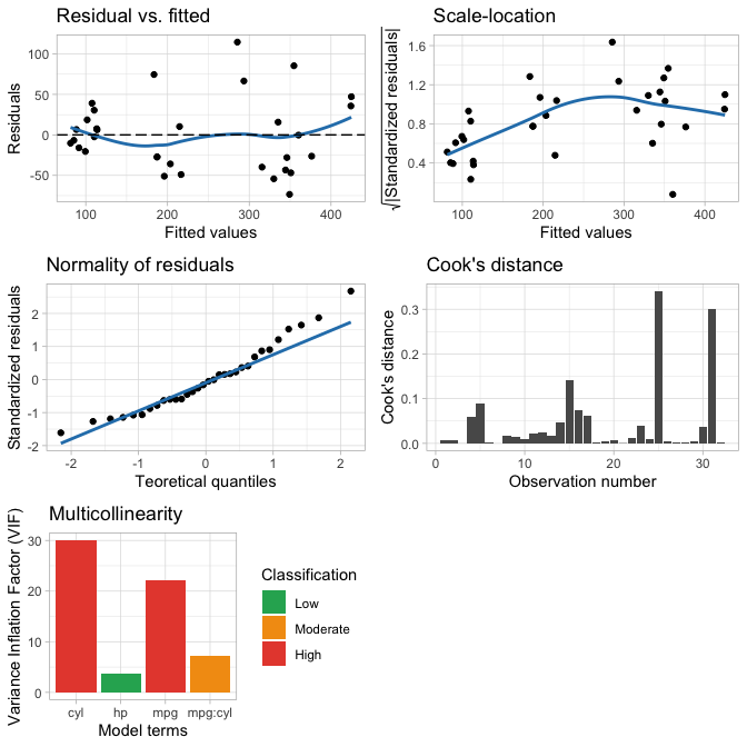
These binaries (installable software) and packages are in development.
They may not be fully stable and should be used with caution. We make no claims about them.
Health stats visible at Monitor.