The hardware and bandwidth for this mirror is donated by dogado GmbH, the Webhosting and Full Service-Cloud Provider. Check out our Wordpress Tutorial.
If you wish to report a bug, or if you are interested in having us mirror your free-software or open-source project, please feel free to contact us at mirror[@]dogado.de.
![]()
![]()
The goal of lineartestr is to contrast the linear
hypothesis of a model:
Using the Domínguez-Lobato test which relies on wild-bootstrap. Also the Ramsey RESET test is implemented.
You can install the released version of lineartestr from
CRAN with:
install.packages("lineartestr")And the development version from GitHub with:
# install.packages("devtools")
devtools::install_github("FedericoGarza/lineartestr")lm functionlibrary(lineartestr)
x <- 1:100
y <- 1:100
lm_model <- lm(y~x)
dl_test <- dominguez_lobato_test(lm_model)dplyr::glimpse(dl_test$test)
#> Observations: 1
#> Variables: 7
#> $ name_distribution <chr> "rnorm"
#> $ name_statistic <chr> "cvm_value"
#> $ statistic <dbl> 7.562182e-29
#> $ p_value <dbl> 0.4066667
#> $ quantile_90 <dbl> 2.549223e-28
#> $ quantile_95 <dbl> 3.887169e-28
#> $ quantile_99 <dbl> 6.359681e-28Also lineartestr can plot the results
plot_dl_test(dl_test)
library(lineartestr)
x_p <- 1:1e5
y_p <- 1:1e5

lm_model_p <- lm(y_p~x_p)

dl_test_p <- dominguez_lobato_test(lm_model_p, n_cores=7)dplyr::glimpse(dl_test_p$test)
#> Observations: 1
#> Variables: 7
#> $ name_distribution <chr> "rnorm"
#> $ name_statistic <chr> "cvm_value"
#> $ statistic <dbl> 6.324343e-21
#> $ p_value <dbl> 0.3566667
#> $ quantile_90 <dbl> 1.902697e-20
#> $ quantile_95 <dbl> 2.532663e-20
#> $ quantile_99 <dbl> 4.141126e-20library(lineartestr)
x <- 1:100 + rnorm(100)
y <- 1:100
lm_model <- lm(y~x)
r_test <- reset_test(lm_model)dplyr::glimpse(r_test)
#> Observations: 1
#> Variables: 6
#> $ statistic <dbl> 0.7797557
#> $ p_value <dbl> 0.6771396
#> $ df <int> 2
#> $ quantile_90 <dbl> 4.60517
#> $ quantile_95 <dbl> 5.991465
#> $ quantile_99 <dbl> 9.21034An then we can plot the results
plot_reset_test(r_test)
lfelibrary(lineartestr)
library(dplyr)
#>
#> Attaching package: 'dplyr'
#> The following objects are masked from 'package:stats':
#>
#> filter, lag
#> The following objects are masked from 'package:base':
#>
#> intersect, setdiff, setequal, union
library(lfe)
#> Loading required package: Matrix
# This example was taken from https://www.rdocumentation.org/packages/lfe/versions/2.8-5/topics/felm
x <- rnorm(1000)
x2 <- rnorm(length(x))
# Individuals and firms
id <- factor(sample(20,length(x),replace=TRUE))
firm <- factor(sample(13,length(x),replace=TRUE))
# Effects for them
id.eff <- rnorm(nlevels(id))
firm.eff <- rnorm(nlevels(firm))
# Left hand side
u <- rnorm(length(x))
y <- x + 0.5*x2 + id.eff[id] + firm.eff[firm] + u
new_y <- y + rnorm(length(y))
## Estimate the model
est <- lfe::felm(y ~ x + x2 | id + firm)
## Testing the linear hypothesis and plotting results
dominguez_lobato_test(est, n_cores = 7) %>%
plot_dl_test()
library(lineartestr)
library(dplyr)

x <- rnorm(100)**3

arma_model <- forecast::Arima(x, order = c(1, 0, 1))
#> Registered S3 method overwritten by 'xts':
#>   method     from
#>   as.zoo.xts zoo
#> Registered S3 method overwritten by 'quantmod':
#>   method            from
#>   as.zoo.data.frame zoo
#> Registered S3 methods overwritten by 'forecast':
#>   method             from
#>   fitted.fracdiff    fracdiff
#>   residuals.fracdiff fracdiff

dominguez_lobato_test(arma_model) %>%
  plot_dl_test()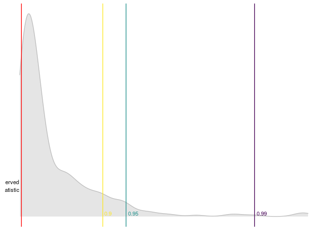
These binaries (installable software) and packages are in development.
They may not be fully stable and should be used with caution. We make no claims about them.
Health stats visible at Monitor.