The hardware and bandwidth for this mirror is donated by dogado GmbH, the Webhosting and Full Service-Cloud Provider. Check out our Wordpress Tutorial.
If you wish to report a bug, or if you are interested in having us mirror your free-software or open-source project, please feel free to contact us at mirror[@]dogado.de.

kindling

Package overview

Title: Higher-Level Interface of ‘torch’ Package to Auto-Train Neural Networks

Whether you’re generating neural network architectures expressions or fitting/training actual models, {kindling} minimizes boilerplate code while preserving {torch}. Since this package uses {torch} as its backend, GPU/TPU devices also supported.

{kindling} also bridges the gap between {torch} and {tidymodels}. It works seamlessly with {parsnip}, {recipes}, and {workflows} to bring deep learning into your existing {tidymodels} modeling pipeline. This enables a streamlined interface for building, training, and tuning deep learning models within the familiar {tidymodels} ecosystem.

Main Features

Code generation of {torch} expression
Multiple architectures available: feedforward networks (MLP/DNN/FFNN) and recurrent variants (RNN, LSTM, GRU)
Native support for titanic ML frameworks (currently supports {tidymodels}, {mlr3} for later) workflows and pipelines
Fine-grained control over network depth, layer sizes, and activation functions
GPU acceleration supports via {torch} tensors

Supported Architectures (As of now)

Feedforward Networks (DNN/FFNN): Classic multi-layer perceptrons for tabular data and general supervised learning
Recurrent Neural Networks (RNN): Basic recurrent architecture for sequential patterns
Long Short-Term Memory (LSTM): Sophisticated recurrent networks with gating mechanisms for long-range dependencies
Gated Recurrent Units (GRU): Streamlined alternative to LSTM with fewer parameters

Installation

You can install {kindling} on CRAN:

install.packages('kindling')

Or install the development version from GitHub:

# install.packages("pak")
pak::pak("joshuamarie/kindling")
## devtools::install_github("joshuamarie/kindling")

Usage: Three Levels of Interaction

{kindling} is powered by R’s metaprogramming capabilities through code generation. Generated torch::nn_module() expressions power the training functions, which in turn serve as engines for {tidymodels} integration. This architecture gives you flexibility to work at whatever abstraction level suits your task.

library(kindling)
#> 
#> Attaching package: 'kindling'
#> The following object is masked from 'package:base':
#> 
#>     args

Before starting, you need to install LibTorch, the backend of PyTorch which also the backend of {torch} R package:

torch::install_torch()

Level 1: Code Generation for `torch::nn_module`

At the lowest level, you can generate raw torch::nn_module code for maximum customization. Functions ending with _generator return unevaluated expressions you can inspect, modify, or execute.

Here’s how to generate a feedforward network specification:

ffnn_generator(
    nn_name = "MyFFNN",
    hd_neurons = c(64, 32, 16),
    no_x = 10,
    no_y = 1,
    activations = 'relu'
)
#> torch::nn_module("MyFFNN", initialize = function () 
#> {
#>     self$fc1 = torch::nn_linear(10, 64, bias = TRUE)
#>     self$fc2 = torch::nn_linear(64, 32, bias = TRUE)
#>     self$fc3 = torch::nn_linear(32, 16, bias = TRUE)
#>     self$out = torch::nn_linear(16, 1, bias = TRUE)
#> }, forward = function (x) 
#> {
#>     x = self$fc1(x)
#>     x = torch::nnf_relu(x)
#>     x = self$fc2(x)
#>     x = torch::nnf_relu(x)
#>     x = self$fc3(x)
#>     x = torch::nnf_relu(x)
#>     x = self$out(x)
#>     x
#> })

This creates a three-hidden-layer network (64 - 32 - 16 neurons) that takes 10 inputs and produces 1 output. Each hidden layer uses ReLU activation, while the output layer remains “untransformed”.

Level 2: Direct Training Interface

Skip the code generation and train models directly with your data. This approach handles all the {torch} boilerplate when training the models internally.

Let’s classify iris species:

model = ffnn(
    Species ~ .,
    data = iris,
    hidden_neurons = c(10, 15, 7),
    activations = act_funs(relu, softshrink = args(lambd = 0.5), elu), 
    loss = "cross_entropy",
    epochs = 100
)

model

======================= Feedforward Neural Networks (MLP) ======================


-- FFNN Model Summary ----------------------------------------------------------

    -----------------------------------------------------------------------
      NN Model Type           :             FFNN    n_predictors :      4
      Number of Epochs        :              100    n_response   :      3
      Hidden Layer Units      :        10, 15, 7    reg.         :   None
      Number of Hidden Layers :                3    Device       :    cpu
      Pred. Type              :   classification                 :       
    -----------------------------------------------------------------------



-- Activation function ---------------------------------------------------------

               -------------------------------------------------
                 1st Layer {10}    :                      relu
                 2nd Layer {15}    :   softshrink(lambd = 0.5)
                 3rd Layer {7}     :                       elu
                 Output Activation :   No act function applied
               -------------------------------------------------

Evaluate the prediction through predict(). The predict() method is extended for fitted models through its newdata argument.

Two kinds of predict() usage:

Without newdata predictions is the default to the parent data frame.

predict(model) |>
    (\(x) table(actual = iris$Species, predicted = x))()
#>             predicted
#> actual       setosa versicolor virginica
#>   setosa         50          0         0
#>   versicolor      0         46         4
#>   virginica       0          2        48

With newdata simply pass the new data frame as the new reference.

sample_iris = dplyr::slice_sample(iris, n = 10, by = Species)

predict(model, newdata = sample_iris) |>
    (\(x) table(actual = sample_iris$Species, predicted = x))()
#>             predicted
#> actual       setosa versicolor virginica
#>   setosa         10          0         0
#>   versicolor      0         10         0
#>   virginica       0          1         9

Level 3: Conventional tidymodels Integration

Work with neural networks just like any other {parsnip} model. This unlocks the entire {tidymodels} toolkit for preprocessing, cross-validation, and model evaluation.

# library(kindling)
# library(parsnip)
# library(yardstick)
box::use(
    kindling[mlp_kindling, rnn_kindling, act_funs, args],
    parsnip[fit, augment],
    yardstick[metrics],
    mlbench[Ionosphere] # data(Ionosphere, package = "mlbench")
)

ionosphere_data = Ionosphere[, -2]

# Train a feedforward network with parsnip
mlp_kindling(
    mode = "classification",
    hidden_neurons = c(128, 64),
    activations = act_funs(relu, softshrink = args(lambd = 0.5)),
    epochs = 100
) |>
    fit(Class ~ ., data = ionosphere_data) |>
    augment(new_data = ionosphere_data) |>
    metrics(truth = Class, estimate = .pred_class)
#> # A tibble: 2 × 3
#>   .metric  .estimator .estimate
#>   <chr>    <chr>          <dbl>
#> 1 accuracy binary         0.989
#> 2 kap      binary         0.975

# Or try a recurrent architecture (demonstrative example with tabular data)
rnn_kindling(
    mode = "classification",
    hidden_neurons = c(128, 64),
    activations = act_funs(relu, elu),
    epochs = 100,
    rnn_type = "gru"
) |>
    fit(Class ~ ., data = ionosphere_data) |>
    augment(new_data = ionosphere_data) |>
    metrics(truth = Class, estimate = .pred_class)
#> # A tibble: 2 × 3
#>   .metric  .estimator .estimate
#>   <chr>    <chr>          <dbl>
#> 1 accuracy binary         0.641
#> 2 kap      binary         0

Hyperparameter Tuning & Resampling

The package has integration with {tidymodels}, so it supports hyperparameter tuning via {tune} with searchable parameters.

The current searchable parameters under {kindling}:

Layer widths (neurons per layer)
Network depth (number of hidden layers)
Activation function combinations
Output activation
Optimizer (Type of optimization algorithm)
Bias (choose between the presence and the absence of the bias term)
Validation Split Proportion
Bidirectional (boolean; only for RNN)

The searchable parameters outside from {kindling}, i.e. under {dials} package such as learn_rate() also supported.

Here’s an example:

# library(tidymodels)
box::use(
    kindling[
        mlp_kindling, hidden_neurons, activations, output_activation, grid_depth
    ],
    parsnip[fit, augment],
    recipes[recipe],
    workflows[workflow, add_recipe, add_model],
    rsample[vfold_cv],
    tune[tune_grid, tune, select_best, finalize_workflow],
    dials[grid_random],
    yardstick[accuracy, roc_auc, metric_set, metrics]
)

mlp_tune_spec = mlp_kindling(
    mode = "classification",
    hidden_neurons = tune(),
    activations = tune(),
    output_activation = tune()
)

iris_folds = vfold_cv(iris, v = 3)
nn_wf = workflow() |>
    add_recipe(recipe(Species ~ ., data = iris)) |>
    add_model(mlp_tune_spec)

nn_grid_depth = grid_depth(
    hidden_neurons(c(32L, 128L)),
    activations(c("relu", "elu")),
    output_activation(c("sigmoid", "linear")),
    n_hlayer = 2,
    size = 10,
    type = "latin_hypercube"
)

# This is supported but limited to 1 hidden layer only
## nn_grid = grid_random(
##     hidden_neurons(c(32L, 128L)),
##     activations(c("relu", "elu")),
##     output_activation(c("sigmoid", "linear")),
##     size = 10
## )

nn_tunes = tune::tune_grid(
    nn_wf,
    iris_folds,
    grid = nn_grid_depth
    # metrics = metric_set(accuracy, roc_auc)
)

best_nn = select_best(nn_tunes)
final_nn = finalize_workflow(nn_wf, best_nn)
# Last run: 4 - 91 (relu) - 3 (sigmoid) units
final_nn_model = fit(final_nn, data = iris)

final_nn_model |>
    augment(new_data = iris) |>
    metrics(truth = Species, estimate = .pred_class)
#> # A tibble: 2 × 3
#>   .metric  .estimator .estimate
#>   <chr>    <chr>          <dbl>
#> 1 accuracy multiclass     0.667
#> 2 kap      multiclass     0.5

Resampling strategies from {rsample} will enable robust cross-validation workflows, orchestrated through the {tune} and {dials} APIs.

Variable Importance

{kindling} integrates with established variable importance methods from {NeuralNetTools} and {vip} to interpret trained neural networks. Two primary algorithms are available:

Garson’s Algorithm

garson(model, bar_plot = FALSE)
#>        x_names y_names  rel_imp
#> 1  Sepal.Width       y 29.04598
#> 2  Petal.Width       y 27.50590
#> 3 Sepal.Length       y 24.20982
#> 4 Petal.Length       y 19.23830

Olden’s Algorithm

olden(model, bar_plot = FALSE)
#>        x_names y_names     rel_imp
#> 1  Sepal.Width       y  0.56231712
#> 2  Petal.Width       y -0.51113650
#> 3 Petal.Length       y -0.29761552
#> 4 Sepal.Length       y -0.06857191

Integration with {vip}

For users working within the {tidymodels} ecosystem, {kindling} models work seamlessly with the {vip} package:

box::use(
    vip[vi, vip]
)

vi(model) |> 
    vip()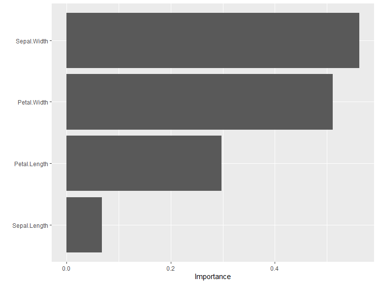

Variable Importance Plot

Note: Weight caching increases memory usage proportional to network size. Only enable it when you plan to compute variable importance multiple times on the same model.

References

Falbel D, Luraschi J (2023). torch: Tensors and Neural Networks with ‘GPU’ Acceleration. R package version 0.13.0, https://torch.mlverse.org, https://github.com/mlverse/torch.

Wickham H (2019). Advanced R, 2nd edition. Chapman and Hall/CRC. ISBN 978-0815384571, https://adv-r.hadley.nz/.

Goodfellow I, Bengio Y, Courville A (2016). Deep Learning. MIT Press. https://www.deeplearningbook.org/.

License

MIT + file LICENSE

Code of Conduct

Please note that the kindling project is released with a Contributor Code of Conduct. By contributing to this project, you agree to abide by its terms.

These binaries (installable software) and packages are in development.
They may not be fully stable and should be used with caution. We make no claims about them.
Health stats visible at Monitor.