The hardware and bandwidth for this mirror is donated by dogado GmbH, the Webhosting and Full Service-Cloud Provider. Check out our Wordpress Tutorial.
If you wish to report a bug, or if you are interested in having us mirror your free-software or open-source project, please feel free to contact us at mirror[@]dogado.de.
jcolors introjcolors contains a selection of ggplot2
color palettes that I like (or can at least tolerate to some degree)
Install jcolors from GitHub:
install.packages("devtools")
devtools::install_github("jaredhuling/jcolors")
Access the jcolors color palettes with
jcolors():
library(jcolors)

jcolors('default')
## kelly_green rich_electric_blue maximum_red majorelle_blue
## "#29BF12" "#00A5CF" "#DE1A1A" "#574AE2"
## fluorescent_orange
## "#FFBF00"display_all_jcolors()
display_all_jcolors_contin()
ggplot2Now use scale_color_jcolors() with
ggplot2:
library(ggplot2)
library(gridExtra)

data(morley)

pltl <- ggplot(data = morley, aes(x = Run, y = Speed,
group = factor(Expt),
colour = factor(Expt))) +
    geom_line(size = 2) +
    theme_bw() +
    theme(panel.background = element_rect(fill = "grey97"),
          panel.border = element_blank(),
          legend.position = "bottom")

pltd <- ggplot(data = morley, aes(x = Run, y = Speed,
group = factor(Expt),
colour = factor(Expt))) +
    geom_line(size = 2) +
    theme_bw() +
    theme(panel.background = element_rect(fill = "grey15"),
          legend.key = element_rect(fill = "grey15"),
          panel.border = element_blank(),
          panel.grid.major = element_line(color = "grey45"),
          panel.grid.minor = element_line(color = "grey25"),
          legend.position = "bottom")

grid.arrange(pltl + scale_color_jcolors(palette = "default"),
             pltd + scale_color_jcolors(palette = "default"), ncol = 2)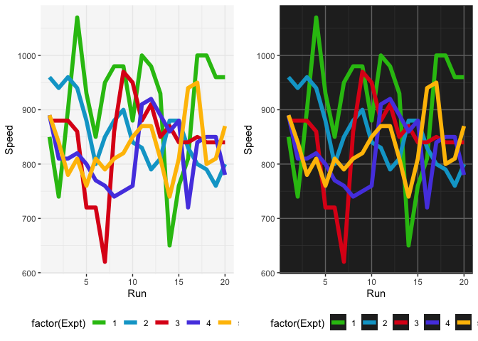
grid.arrange(pltl + scale_color_jcolors(palette = "pal2"),
             pltd + scale_color_jcolors(palette = "pal2"), ncol = 2)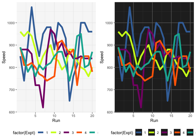
Color palettes can be displayed using
display_jcolors()
display_jcolors("default")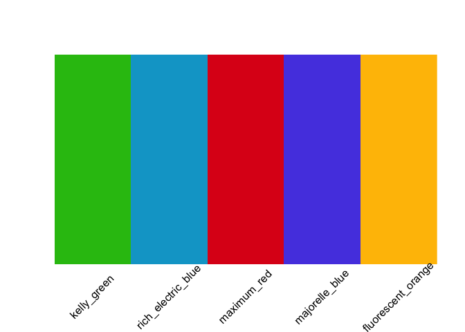
display_jcolors("pal2")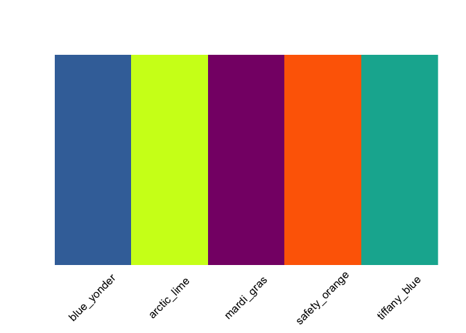
display_jcolors("pal3")
display_jcolors("pal4")
display_jcolors("pal5")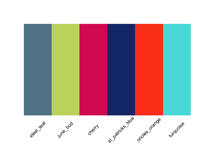
display_jcolors("pal6")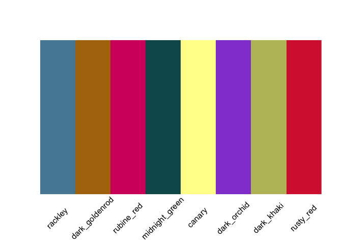
display_jcolors("pal7")
display_jcolors("pal8")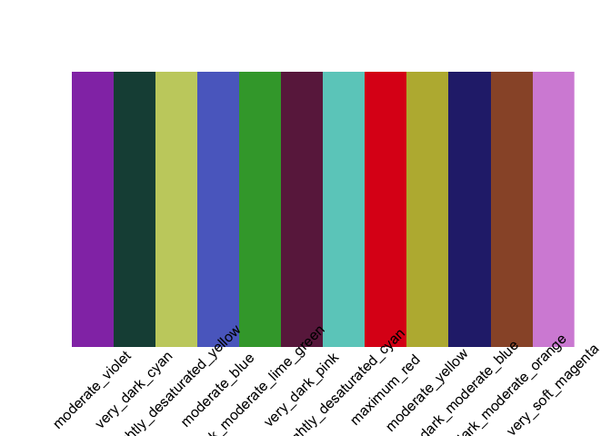
display_jcolors("pal9")
display_jcolors("pal10")
display_jcolors("pal11")
display_jcolors("pal12")
display_jcolors("rainbow")
grid.arrange(pltl + scale_color_jcolors(palette = "pal3"),
             pltd + scale_color_jcolors(palette = "pal3"), ncol = 2)
grid.arrange(pltl + scale_color_jcolors(palette = "pal4"),
             pltd + scale_color_jcolors(palette = "pal4") +
                 theme(panel.background = element_rect(fill = "grey5")), ncol = 2)
grid.arrange(pltl + scale_color_jcolors(palette = "pal5"),
             pltd + scale_color_jcolors(palette = "pal5"), ncol = 2)
pltd <- ggplot(data = OrchardSprays, aes(x = rowpos, y = decrease,
group = factor(treatment),
colour = factor(treatment))) +
    geom_line(size = 2) +
    geom_point(size = 4) +
    theme_bw() +
    theme(panel.background = element_rect(fill = "grey15"),
          legend.key = element_rect(fill = "grey15"),
          panel.border = element_blank(),
          panel.grid.major = element_line(color = "grey45"),
          panel.grid.minor = element_line(color = "grey25"),
          legend.position = "bottom")


pltd + scale_color_jcolors(palette = "pal6")
display_all_jcolors_contin()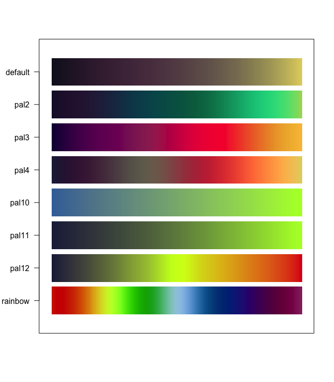
ggplot2set.seed(42)
plt <- ggplot(data.frame(x = rnorm(10000), y = rexp(10000, 1.5)), aes(x = x, y = y)) +
geom_hex() + coord_fixed() + theme(legend.position = "bottom")
plt2 <- plt + scale_fill_jcolors_contin("pal2", bias = 1.75) + theme_bw()
plt3 <- plt + scale_fill_jcolors_contin("pal3", reverse = TRUE, bias = 2.25) + theme_bw()
plt4 <- plt + scale_fill_jcolors_contin("pal12", reverse = TRUE, bias = 2) + theme_bw()
grid.arrange(plt2, plt3, plt4, ncol = 2)
ggplot2 themeslibrary(scales)
p1 <- ggplot(aes(x = carat, y = price), data = diamonds) +
geom_point(alpha = 0.5, size = 1, aes(color = clarity)) +
scale_x_continuous(trans = log10_trans(), limits = c(0.2, 3),
breaks = c(0.2, 0.5, 1, 2, 3)) +
scale_y_continuous(trans = log10_trans(), limits = c(350, 15000),
breaks = c(350, 1000, 5000, 10000, 15000)) +
ggtitle('Price (log10) by Carat (log10) and Clarity') +
scale_color_jcolors("rainbow") +
theme_light_bg()
p2 <- ggplot(aes(x = carat, y = price), data = diamonds) +
geom_point(alpha = 0.5, size = 1, aes(color = cut)) +
scale_x_continuous(trans = log10_trans(), limits = c(0.2, 3),
breaks = c(0.2, 0.5, 1, 2, 3)) +
scale_y_continuous(trans = log10_trans(), limits = c(350, 15000),
breaks = c(350, 1000, 5000, 10000, 15000)) +
ggtitle('Price (log10) by Carat (log10) and Cut') +
scale_color_jcolors("pal4") +
theme_light_bg()
grid.arrange(p1, p2, ncol = 2)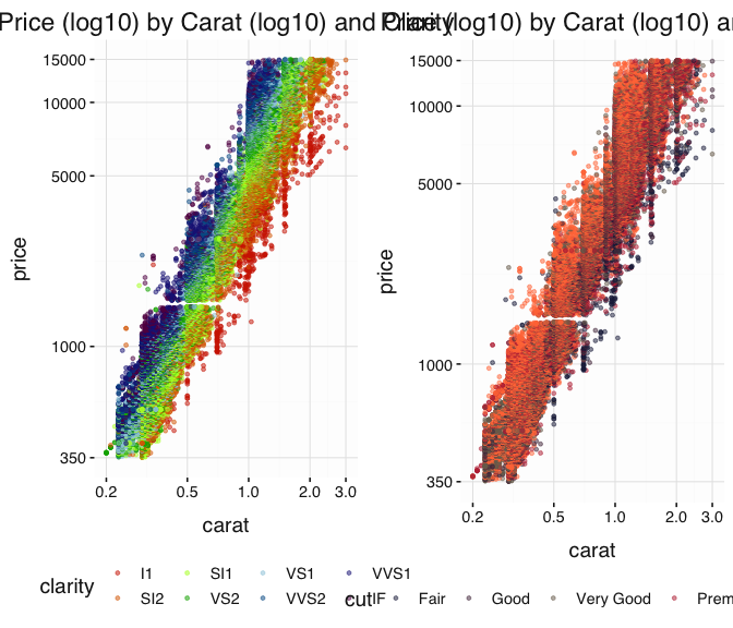
p1 <- ggplot(aes(x = clarity, y = price), data = diamonds) +
      geom_point(alpha = 0.25, size = 1, position = "jitter", aes(color = log(carat + 1))) +
      scale_y_continuous(trans = log10_trans(), limits = c(350, 15000),
        breaks = c(350, 1000, 5000, 10000, 15000)) +
      ggtitle('Price (log10) by Carat (log10) and Clarity')

p2 <- ggplot(aes(x = clarity, y = price), data = diamonds) +
      geom_point(alpha = 0.25, size = 1, position = "jitter", aes(color = log(carat + 1))) +
      scale_y_continuous(trans = log10_trans(), limits = c(350, 15000),
        breaks = c(350, 1000, 5000, 10000, 15000)) +
      ggtitle('Price (log10) by Carat (log10) and Clarity')

grid.arrange(p1 + scale_color_jcolors_contin("pal3", bias = 1.75) + theme_light_bg(),
             p2 + scale_color_jcolors_contin("rainbow") + theme_light_bg(), ncol = 2)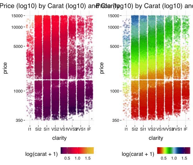
If the background here were dark, then this would look nice:
grid.arrange(p1 + scale_color_jcolors_contin("pal3", bias = 1.75) + theme_dark_bg(),
             p2 + scale_color_jcolors_contin("rainbow") + theme_dark_bg(), ncol = 2)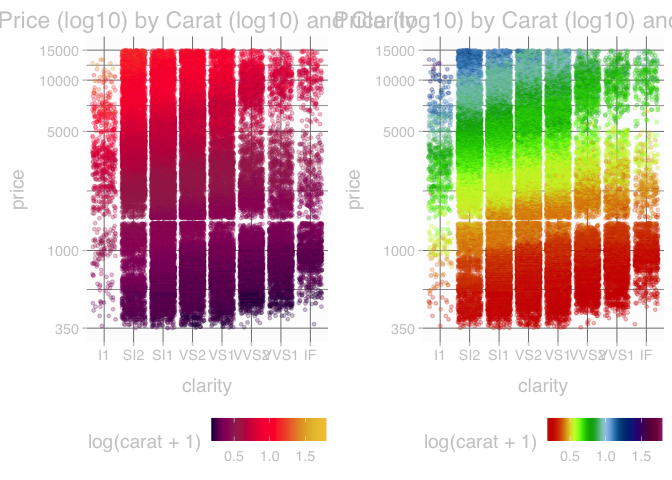
These binaries (installable software) and packages are in development.
They may not be fully stable and should be used with caution. We make no claims about them.
Health stats visible at Monitor.