The hardware and bandwidth for this mirror is donated by dogado GmbH, the Webhosting and Full Service-Cloud Provider. Check out our Wordpress Tutorial.
If you wish to report a bug, or if you are interested in having us mirror your free-software or open-source project, please feel free to contact us at mirror[@]dogado.de.
![]()
![]()
The goal of healthyR is to help quickly analyze common data problems in the Administrative and Clincial spaces.
You can install the released version of healthyR from CRAN with:
install.packages("healthyR")And the development version from GitHub with:
# install.packages("devtools")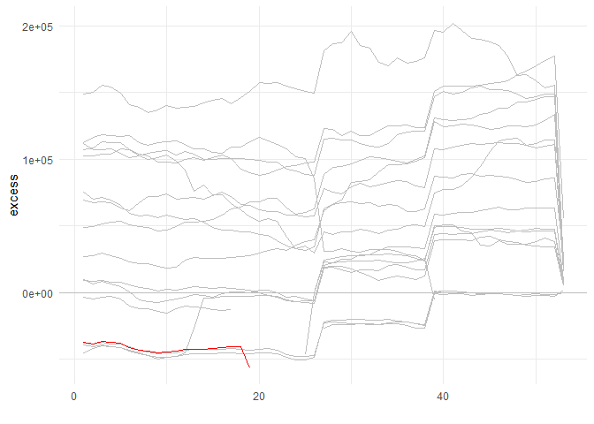
devtools::install_github("spsanderson/healthyR")This is a basic example of using the ts_median_excess_plt() function`:
library(healthyR)
library(timetk)
library(dplyr)

ts_signature_tbl(.data = m4_daily, .date_col = date, .pad_time = TRUE, id) %>%
    ts_median_excess_plt(
        .date_col           = date
        , .value_col        = value
        , .x_axis           = week
        , .ggplot_group_var = year
        , .years_back       = 5
    )
Here is a simple example of using the ts_signature_tbl() function:
library(healthyR)
library(timetk)
ts_signature_tbl(.data = m4_daily, .date_col = date)
#> # A tibble: 17,578 × 31
#> id date value index.num diff year year.iso half quarter month
#> <fct> <date> <dbl> <dbl> <dbl> <int> <int> <int> <int> <int>
#> 1 D410 1978-06-23 9109. 267408000 NA 1978 1978 1 2 6
#> 2 D410 1978-06-24 9103. 267494400 86400 1978 1978 1 2 6
#> 3 D410 1978-06-25 9116. 267580800 86400 1978 1978 1 2 6
#> 4 D410 1978-06-26 9116. 267667200 86400 1978 1978 1 2 6
#> 5 D410 1978-06-27 9106. 267753600 86400 1978 1978 1 2 6
#> 6 D410 1978-06-28 9094. 267840000 86400 1978 1978 1 2 6
#> 7 D410 1978-06-29 9094. 267926400 86400 1978 1978 1 2 6
#> 8 D410 1978-06-30 9084. 268012800 86400 1978 1978 1 2 6
#> 9 D410 1978-07-01 9081. 268099200 86400 1978 1978 2 3 7
#> 10 D410 1978-07-02 9047. 268185600 86400 1978 1978 2 3 7
#> # ℹ 17,568 more rows
#> # ℹ 21 more variables: month.xts <int>, month.lbl <ord>, day <int>, hour <int>,
#> # minute <int>, second <int>, hour12 <int>, am.pm <int>, wday <int>,
#> # wday.xts <int>, wday.lbl <ord>, mday <int>, qday <int>, yday <int>,
#> # mweek <int>, week <int>, week.iso <int>, week2 <int>, week3 <int>,
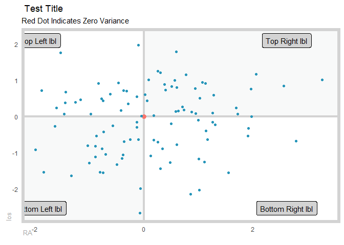
#> # week4 <int>, mday7 <int>Here is a simple example of using the plt_gartner_magic_chart() function:
suppressPackageStartupMessages(library(healthyR))
suppressPackageStartupMessages(library(tibble))
suppressPackageStartupMessages(library(dplyr))

gartner_magic_chart_plt(
  .data = tibble(x = rnorm(100, 0, 1), y = rnorm(100, 0, 1))
  , .x_col = x
  , .y_col = y
  , .y_lab = "los"
  , .x_lab = "RA"
  , .plot_title = "Test Title"
  , .top_left_label = "Top Left lbl"
  , .top_right_label = "Top Right lbl"
  , .bottom_left_label = "Bottom Left lbl"
  , .bottom_right_label = "Bottom Right lbl"
)
These binaries (installable software) and packages are in development.
They may not be fully stable and should be used with caution. We make no claims about them.
Health stats visible at Monitor.