The hardware and bandwidth for this mirror is donated by dogado GmbH, the Webhosting and Full Service-Cloud Provider. Check out our Wordpress Tutorial.
If you wish to report a bug, or if you are interested in having us mirror your free-software or open-source project, please feel free to contact us at mirror[@]dogado.de.
The goal of healthyR.ts is to provide a consistent verb framework for performing time series analysis and forecasting on both administrative and clinical hospital data.
You can install the released version of healthyR.ts from CRAN with:
And the development version from GitHub with:
This is a basic example which shows you how to generate random walk data.
library(healthyR.ts)
library(ggplot2)

df <- ts_random_walk()

head(df)
#> # A tibble: 6 × 4
#>     run     x        y cum_y
#>   <dbl> <dbl>    <dbl> <dbl>
#> 1     1     1  0.0541  1054.
#> 2     1     2 -0.143    904.
#> 3     1     3 -0.0285   878.
#> 4     1     4  0.245   1093.
#> 5     1     5  0.0658  1165.
#> 6     1     6  0.00266 1168.
Now that the data has been generated, lets take a look at it.
df %>%
   ggplot(
       mapping = aes(
           x = x
           , y = cum_y
           , color = factor(run)
           , group = factor(run)
        )
    ) +
    geom_line(alpha = 0.8) +
    ts_random_walk_ggplot_layers(df)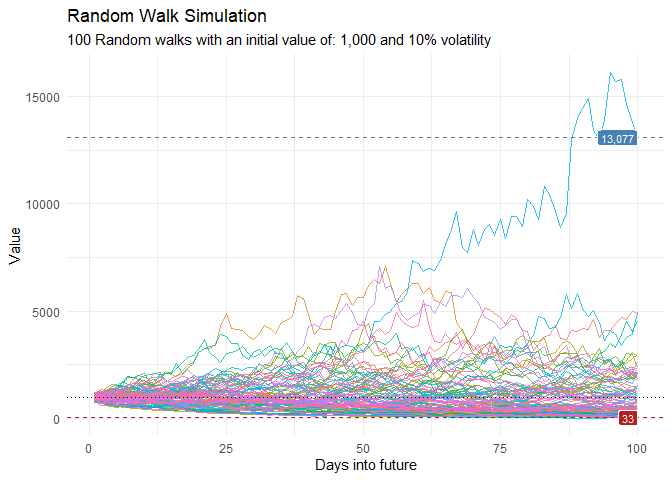
That is still pretty noisy, so lets see this in a different way. Lets clear this up a bit to make it easier to see the full range of the possible volatility of the random walks.
library(dplyr)
library(ggplot2)

df %>%
    group_by(x) %>%
    summarise(
        min_y = min(cum_y),
        max_y = max(cum_y)
    ) %>%
    ggplot(
        aes(x = x)
    ) +
    geom_line(aes(y = max_y), color = "steelblue") +
    geom_line(aes(y = min_y), color = "firebrick") +
    geom_ribbon(aes(ymin = min_y, ymax = max_y), alpha = 0.2) +
    ts_random_walk_ggplot_layers(df)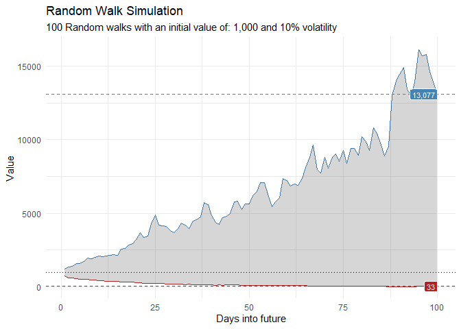
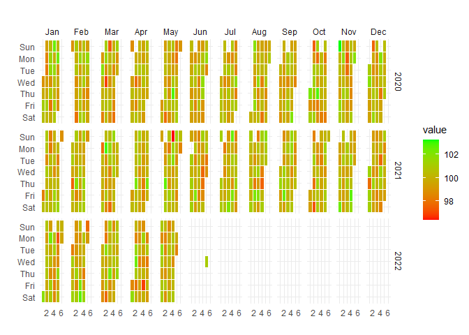
This package comes with a wide variety of functions from Data Generators to Statistics functions. The function ts_random_walk() in the above example is a Data Generator.
Let’s take a look at a plotting function.
data_tbl <- data.frame(
  date_col = seq.Date(
    from = as.Date("2020-01-01"),
    to   = as.Date("2022-06-01"),
    length.out = 365*2 + 180
    ),
  value = rnorm(365*2+180, mean = 100)
)

ts_calendar_heatmap_plot(
  .data          = data_tbl
  , .date_col    = date_col
  , .value_col   = value
  , .interactive = FALSE
)
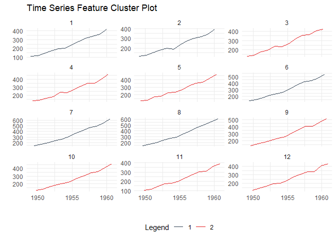
Time Series Clustering via Features:
data_tbl <- ts_to_tbl(AirPassengers) %>%
  mutate(group_id = rep(1:12, 12))

output <- ts_feature_cluster(
  .data = data_tbl,
  .date_col = date_col,
  .value_col = value,
  group_id,
  .features = c("acf_features","entropy"),
  .scale = TRUE,
  .prefix = "ts_",
  .centers = 3
)

ts_feature_cluster_plot(
  .data = output,
  .date_col = date_col,
  .value_col = value,
  .center = 2,
  group_id
)
Time to/from Event Analysis
library(dplyr)
df <- ts_to_tbl(AirPassengers) %>% select(-index)

ts_time_event_analysis_tbl(
  .data = df,
  .horizon = 6,
  .date_col = date_col,
  .value_col = value,
  .direction = "both"
) %>%
  ts_event_analysis_plot()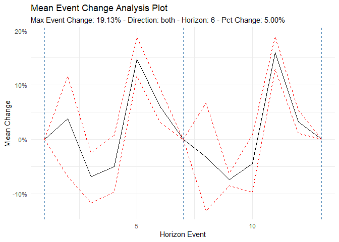
ts_time_event_analysis_tbl(
  .data = df,
  .horizon = 6,
  .date_col = date_col,
  .value_col = value,
  .direction = "both"
) %>%
  ts_event_analysis_plot(.plot_type = "individual")
ARIMA Simulators
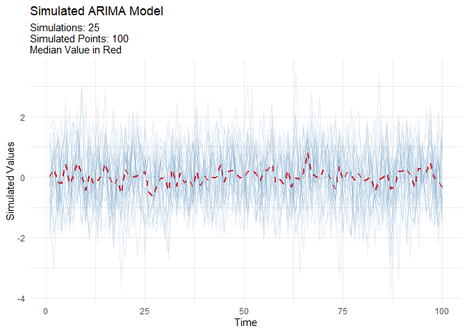
Automatic Workflows which can be thought of as Boiler Plate Time Series modeling. This is in it’s infancy in this package.
| Auto Workflows | Boilerplate Workflow |
|---|---|
| ts_auto_arima() | Boilerplate Workflow |
| ts_auto_arima_xgboost() | Boilerplate Workflow |
| ts_auto_croston() | Boilerplate Workflow |
| ts_auto_exp_smoothing() | Boilerplate Workflow |
| ts_auto_glmnet() | Boilerplate Workflow |
| ts_auto_lm() | Boilerplate Workflow |
| ts_auto_mars() | Boilerplate Workflow |
| ts_auto_nnetar() | Boilerplate Workflow |
| ts_auto_prophet_boost() | Boilerplate Workflow |
| ts_auto_prophet_reg() | Boilerplate Workflow |
| ts_auto_smooth_es() | Boilerplate Workflow |
| ts_auto_svm_poly() | Boilerplate Workflow |
| ts_auto_svm_rbf() | Boilerplate Workflow |
| ts_auto_theta() | Boilerplate Workflow |
| ts_auto_xgboost() | Boilerplate Workflow |
This is just a start of what is in this package!
These binaries (installable software) and packages are in development.
They may not be fully stable and should be used with caution. We make no claims about them.
Health stats visible at Monitor.