The hardware and bandwidth for this mirror is donated by dogado GmbH, the Webhosting and Full Service-Cloud Provider. Check out our Wordpress Tutorial.
If you wish to report a bug, or if you are interested in having us mirror your free-software or open-source project, please feel free to contact us at mirror[@]dogado.de.
![]()
![]()
![]()
Tidy, analyze, and plot causal directed acyclic graphs (DAGs).
ggdag uses the powerful dagitty package to
create and analyze structural causal models and plot them using
ggplot2 and ggraph in a consistent and easy
manner.
You can install ggdag with:
install.packages("ggdag")Or you can install the development version from GitHub with:
# install.packages("devtools")
devtools::install_github("r-causal/ggdag")ggdag makes it easy to use dagitty in the
context of the tidyverse. You can directly tidy dagitty
objects or use convenience functions to create DAGs using a more R-like
syntax:
library(ggdag)
library(ggplot2)

#  example from the dagitty package
dag <- dagitty::dagitty("dag {
    y <- x <- z1 <- v -> z2 -> y
    z1 <- w1 <-> w2 -> z2
    x <- w1 -> y
    x <- w2 -> y
    x [exposure]
    y [outcome]
  }")

tidy_dag <- tidy_dagitty(dag)

tidy_dag
#> # A DAG with 7 nodes and 12 edges
#> #
#> # Exposure: x
#> # Outcome: y
#> #
#> # A tibble: 13 × 8
#>    name       x      y direction to       xend   yend circular
#>    <chr>  <dbl>  <dbl> <fct>     <chr>   <dbl>  <dbl> <lgl>
#>  1 v     0.496  -3.40  ->        z1     1.83   -2.92  FALSE
#>  2 v     0.496  -3.40  ->        z2     0.0188 -2.08  FALSE
#>  3 w1    1.73   -1.94  ->        x      2.07   -1.42  FALSE
#>  4 w1    1.73   -1.94  ->        y      1.00   -0.944 FALSE
#>  5 w1    1.73   -1.94  ->        z1     1.83   -2.92  FALSE
#>  6 w1    1.73   -1.94  <->       w2     0.873  -1.56  FALSE
#>  7 w2    0.873  -1.56  ->        x      2.07   -1.42  FALSE
#>  8 w2    0.873  -1.56  ->        y      1.00   -0.944 FALSE
#>  9 w2    0.873  -1.56  ->        z2     0.0188 -2.08  FALSE
#> 10 x     2.07   -1.42  ->        y      1.00   -0.944 FALSE
#> 11 y     1.00   -0.944 <NA>      <NA>  NA      NA     FALSE
#> 12 z1    1.83   -2.92  ->        x      2.07   -1.42  FALSE
#> 13 z2    0.0188 -2.08  ->        y      1.00   -0.944 FALSE

#  using more R-like syntax to create the same DAG
tidy_ggdag <- dagify(
  y ~ x + z2 + w2 + w1,
  x ~ z1 + w1 + w2,
  z1 ~ w1 + v,
  z2 ~ w2 + v,
  w1 ~ ~w2, # bidirected path
  exposure = "x",
  outcome = "y"
) %>%
  tidy_dagitty()

tidy_ggdag
#> # A DAG with 7 nodes and 12 edges
#> #
#> # Exposure: x
#> # Outcome: y
#> #
#> # A tibble: 13 × 8
#>    name      x     y direction to     xend  yend circular
#>    <chr> <dbl> <dbl> <fct>     <chr> <dbl> <dbl> <lgl>
#>  1 v     -3.58  3.30 ->        z1    -4.05  4.63 FALSE
#>  2 v     -3.58  3.30 ->        z2    -2.23  3.74 FALSE
#>  3 w1    -3.03  5.74 ->        x     -3.20  5.14 FALSE
#>  4 w1    -3.03  5.74 ->        y     -1.98  5.22 FALSE
#>  5 w1    -3.03  5.74 ->        z1    -4.05  4.63 FALSE
#>  6 w1    -3.03  5.74 <->       w2    -2.35  4.72 FALSE
#>  7 w2    -2.35  4.72 ->        x     -3.20  5.14 FALSE
#>  8 w2    -2.35  4.72 ->        y     -1.98  5.22 FALSE
#>  9 w2    -2.35  4.72 ->        z2    -2.23  3.74 FALSE
#> 10 x     -3.20  5.14 ->        y     -1.98  5.22 FALSE
#> 11 y     -1.98  5.22 <NA>      <NA>  NA    NA    FALSE
#> 12 z1    -4.05  4.63 ->        x     -3.20  5.14 FALSE
#> 13 z2    -2.23  3.74 ->        y     -1.98  5.22 FALSE
ggdag also provides functionality for analyzing DAGs and
plotting them in ggplot2:
ggdag(tidy_ggdag) +
  theme_dag()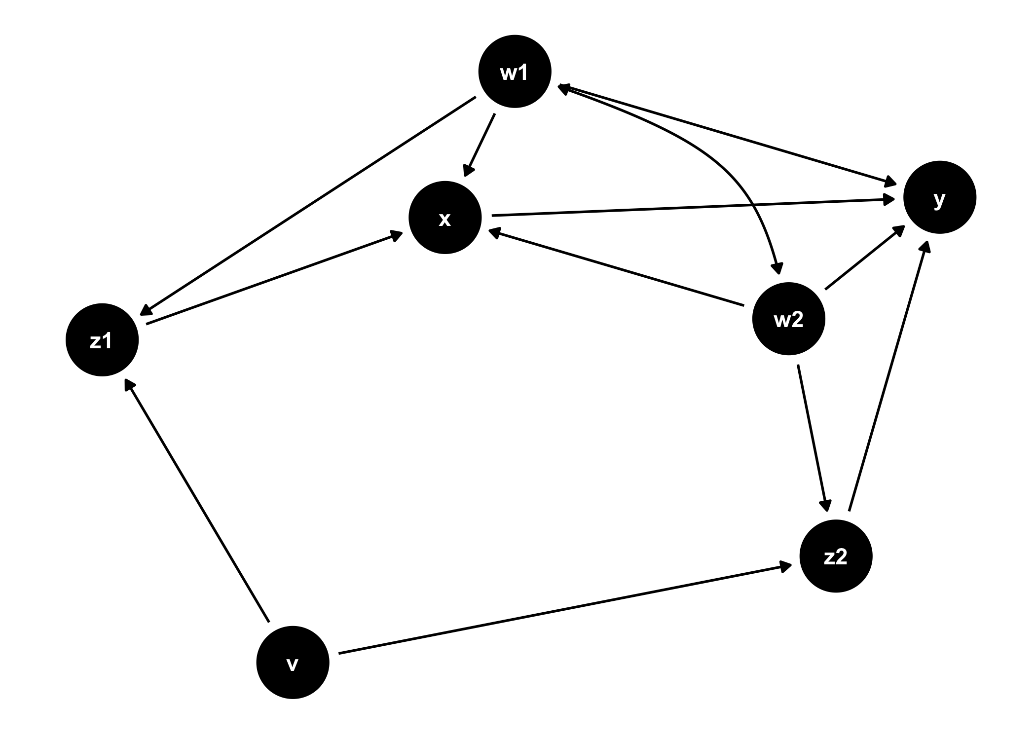
ggdag_adjustment_set(tidy_ggdag, node_size = 14) +
  theme(legend.position = "bottom")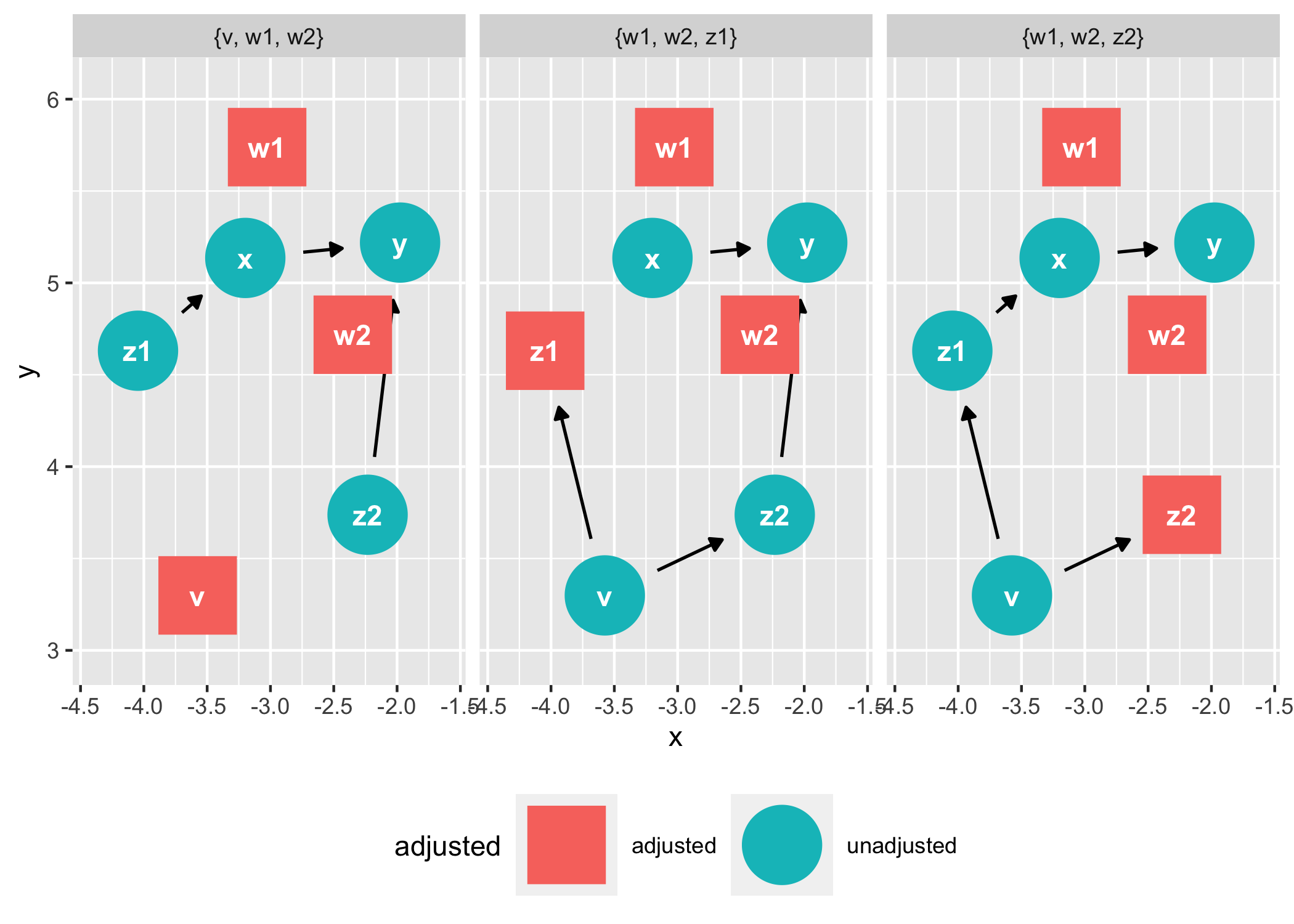
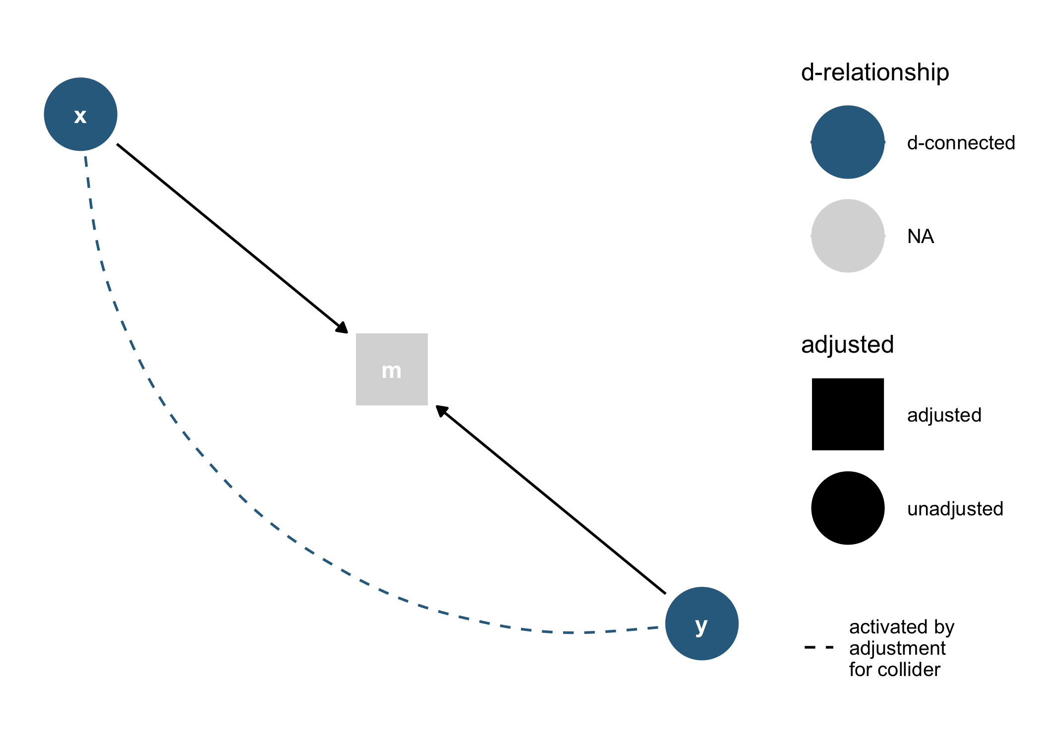
As well as geoms and other functions for plotting them directly in
ggplot2:
dagify(m ~ x + y) %>%
  tidy_dagitty() %>%
  node_dconnected("x", "y", controlling_for = "m") %>%
  ggplot(aes(
    x = x,
    y = y,
    xend = xend,
    yend = yend,
    shape = adjusted,
    col = d_relationship
  )) +
  geom_dag_edges(end_cap = ggraph::circle(10, "mm")) +
  geom_dag_collider_edges() +
  geom_dag_point() +
  geom_dag_text(col = "white") +
  theme_dag() +
  scale_adjusted() +
  expand_plot(expand_y = expansion(c(0.2, 0.2))) +
  scale_color_viridis_d(
    name = "d-relationship",
    na.value = "grey85",
    begin = .35
  )
And common structures of bias:
ggdag_equivalent_dags(confounder_triangle())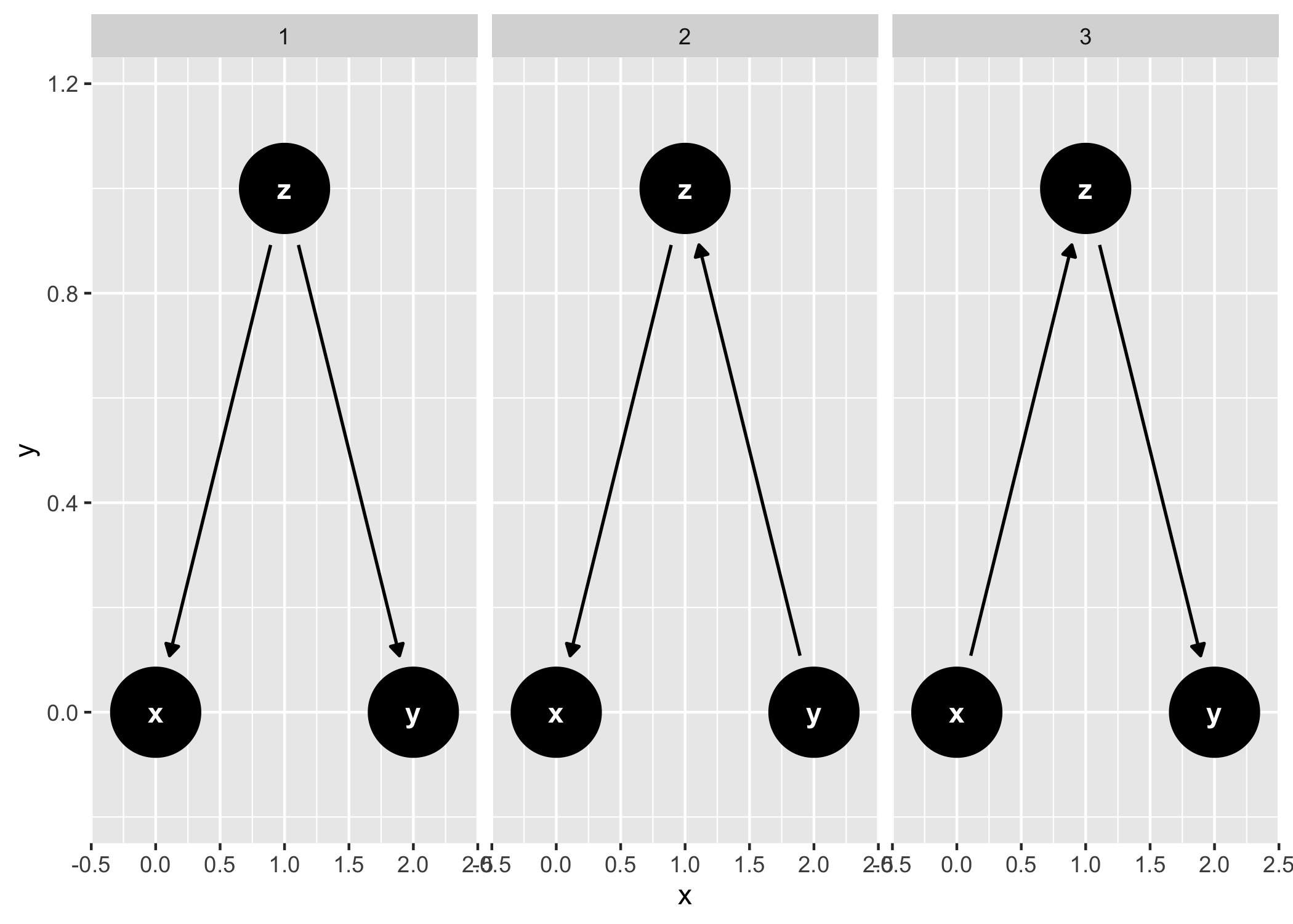
ggdag_butterfly_bias(edge_type = "diagonal")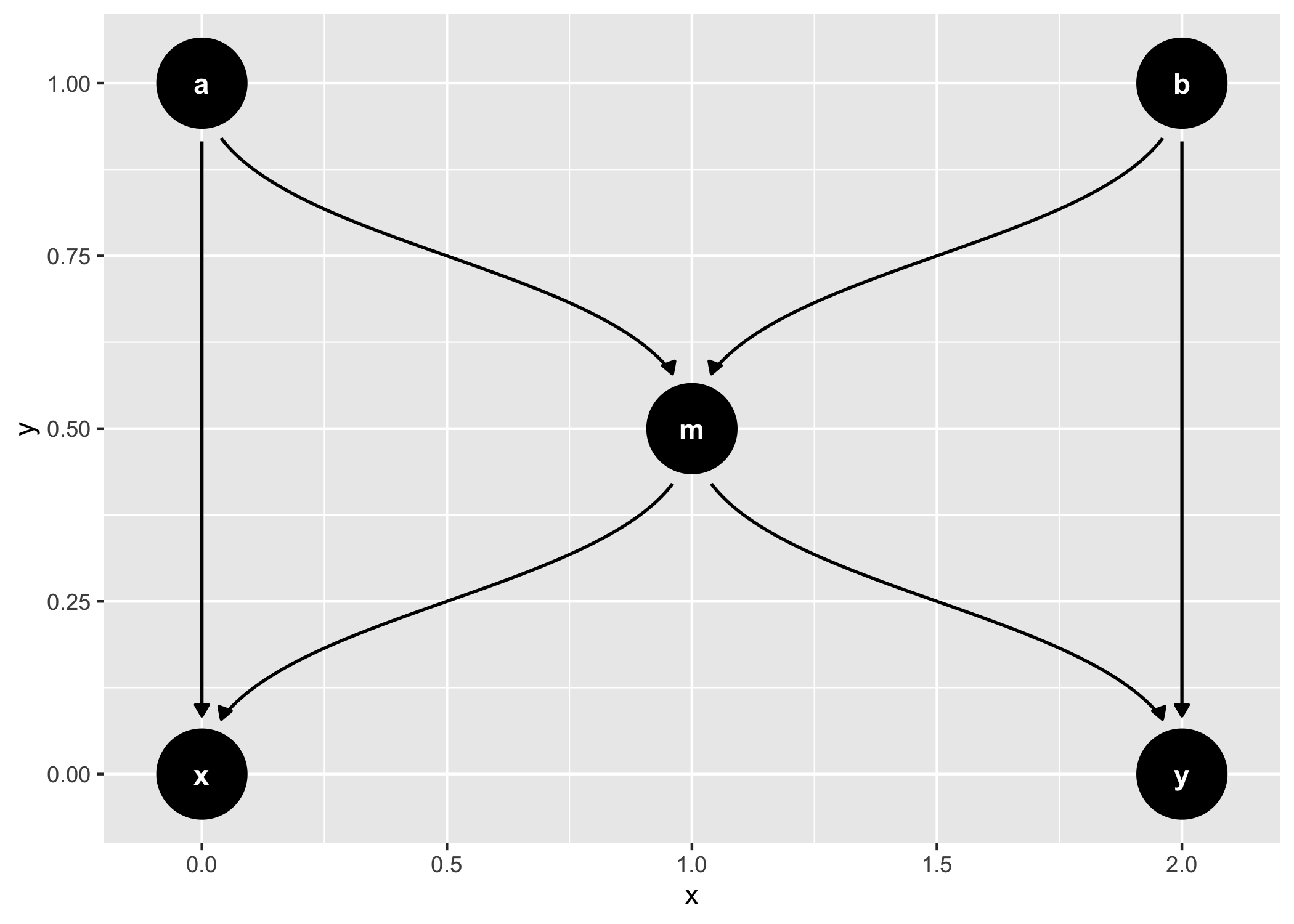
These binaries (installable software) and packages are in development.
They may not be fully stable and should be used with caution. We make no claims about them.
Health stats visible at Monitor.