The hardware and bandwidth for this mirror is donated by dogado GmbH, the Webhosting and Full Service-Cloud Provider. Check out our Wordpress Tutorial.
If you wish to report a bug, or if you are interested in having us mirror your free-software or open-source project, please feel free to contact us at mirror[@]dogado.de.

![]()
![]()

![]()
gaussplotR provides functions to fit two-dimensional
Gaussian functions, predict values from such functions, and produce
plots of predicted data.
You can install gaussplotR from CRAN via:
install.packages("gaussplotR")Or to get the latest (developmental) version through GitHub, use:
devtools::install_github("vbaliga/gaussplotR")The function fit_gaussian_2D() is the workhorse of
gaussplotR. It uses stats::nls() to find the
best-fitting parameters of a 2D-Gaussian fit to supplied data based on
one of three formula choices. The function
autofit_gaussian_2D() can be used to automatically figure
out the best formula choice and arrive at the best-fitting
parameters.
The predict_gaussian_2D() function can then be used to
predict values from the Gaussian over a supplied grid of X- and Y-values
(generated here via expand.grid()). This is useful if the
original data is relatively sparse and interpolation of values is
desired.
Plotting can then be achieved via ggplot_gaussian_2D(),
but note that the data.frame created by
predict_gaussian_2D() can be supplied to other plotting
frameworks such as lattice::levelplot(). A 3D plot can also
be produced via rgl_gaussian_2D() (not shown here).
library(gaussplotR)

## Load the sample data set
data(gaussplot_sample_data)

## The raw data we'd like to use are in columns 1:3
samp_dat <-
  gaussplot_sample_data[,1:3]


#### Example 1: Unconstrained elliptical ####
## This fits an unconstrained elliptical by default
gauss_fit_ue <-
  fit_gaussian_2D(samp_dat)

## Generate a grid of X- and Y- values on which to predict
grid <-
  expand.grid(X_values = seq(from = -5, to = 0, by = 0.1),
              Y_values = seq(from = -1, to = 4, by = 0.1))

## Predict the values using predict_gaussian_2D
gauss_data_ue <-
  predict_gaussian_2D(
    fit_object = gauss_fit_ue,
    X_values = grid$X_values,
    Y_values = grid$Y_values,
  )

## Plot via ggplot2 and metR
library(ggplot2); library(metR)
#> Warning: package 'ggplot2' was built under R version 4.0.5
#> Warning: package 'metR' was built under R version 4.0.5
ggplot_gaussian_2D(gauss_data_ue)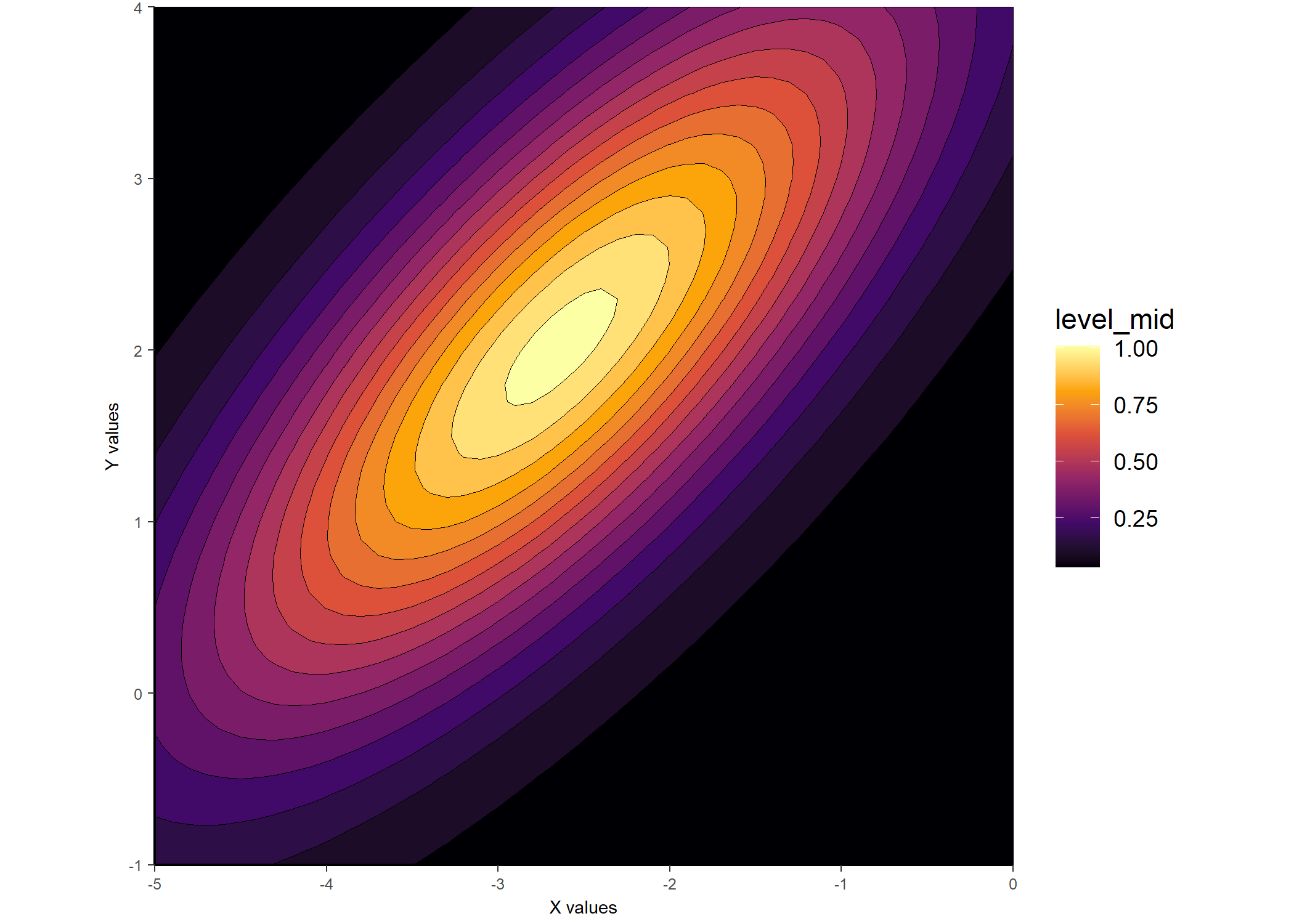
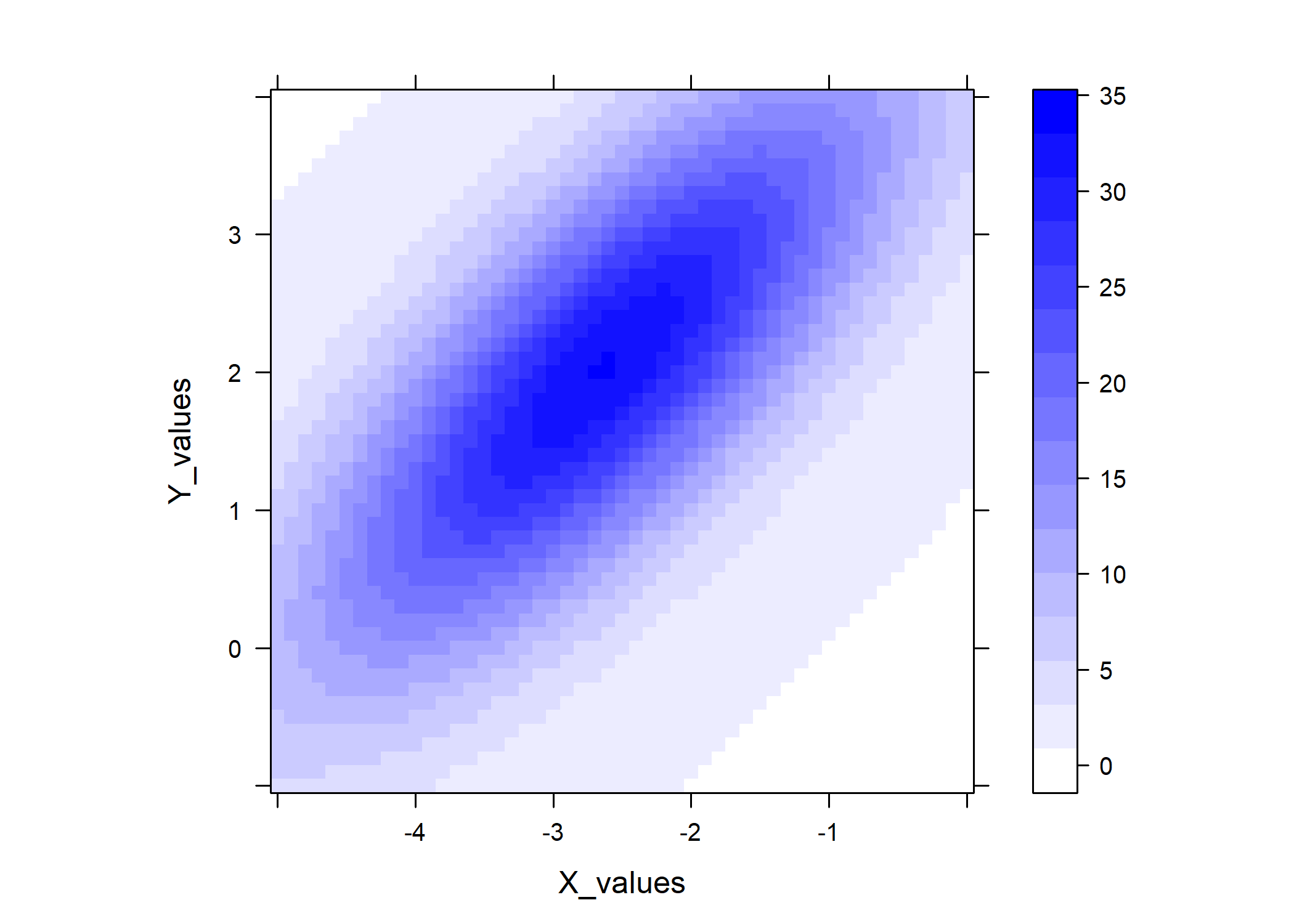
## And another example plot via lattice::levelplot()
library(lattice)
lattice::levelplot(
  predicted_values ~ X_values * Y_values,
  data = gauss_data_ue,
  col.regions = colorRampPalette(
    c("white", "blue")
    )(100),
  asp = 1
)
#### Example 2: Constrained elliptical_log ####
## This fits a constrained elliptical, as in Priebe et al. 2003
gauss_fit_cel <-
  fit_gaussian_2D(
    samp_dat,
    method = "elliptical_log",
    constrain_orientation = -1
  )

## Generate a grid of x- and y- values on which to predict
grid <-
  expand.grid(X_values = seq(from = -5, to = 0, by = 0.1),
              Y_values = seq(from = -1, to = 4, by = 0.1))

## Predict the values using predict_gaussian_2D
gauss_data_cel <-
  predict_gaussian_2D(
    fit_object = gauss_fit_cel,
    X_values = grid$X_values,
    Y_values = grid$Y_values,
  )

## Plot via ggplot2 and metR
ggplot_gaussian_2D(gauss_data_cel)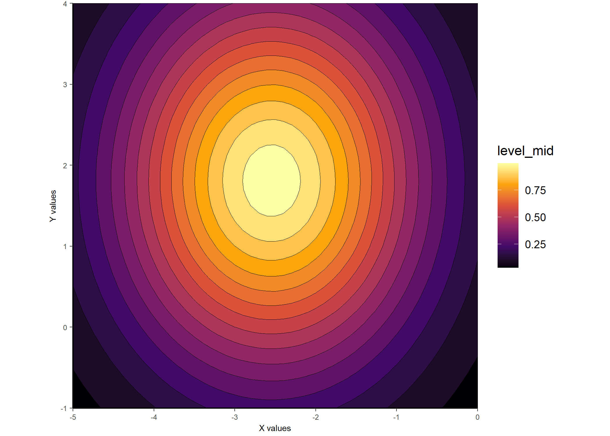
Should you be interested in having gaussplotR try to
automatically determine the best choice of method for
fit_gaussian_2D(), the autofit_gaussian_2D()
function can come in handy. The default is to select the
method that produces a fit with the lowest
rmse, but other choices include rss and
AIC.
## Use autofit_gaussian_2D() to automatically decide the best
## model to use
gauss_auto <-
  autofit_gaussian_2D(
    samp_dat,
    comparison_method = "rmse",
    simplify = TRUE
    )

## The output has the same components as `fit_gaussian_2D()`
## but for the automatically-selected best-fitting method only:
summary(gauss_auto)
#> Model coefficients
#>   A_o   Amp theta X_peak Y_peak    a    b
#>  0.83 32.25  3.58  -2.64   2.02 0.91 0.96
#> Model error stats
#>     rss rmse deviance AIC
#>  156.23 2.08   156.23 171
#> Fitting methods
#>          method       amplitude     orientation
#> "elliptical" "unconstrained" "unconstrained"Feedback on bugs, improvements, and/or feature requests are all welcome. Please see the Issues templates on GitHub to make a bug fix request or feature request.
To contribute code via a pull request, please consult the Contributing Guide first.
Baliga, VB. 2021. gaussplotR: Fit, predict, and plot 2D-Gaussians in R. Journal of Open Source Software, 6(60), 3074. https://doi.org/10.21105/joss.03074
GPL (>= 3) + file LICENSE
🐢
These binaries (installable software) and packages are in development.
They may not be fully stable and should be used with caution. We make no claims about them.
Health stats visible at Monitor.