The hardware and bandwidth for this mirror is donated by dogado GmbH, the Webhosting and Full Service-Cloud Provider. Check out our Wordpress Tutorial.
If you wish to report a bug, or if you are interested in having us mirror your free-software or open-source project, please feel free to contact us at mirror[@]dogado.de.

flexhaz

Dynamic Failure Rate Distributions for Survival Analysis

Capacitors that wear out faster than any Weibull can describe. Software systems with bathtub-shaped crash rates. Post-surgical patients whose risk drops sharply, then slowly climbs again. Standard parametric survival families cannot express these hazard patterns — but flexhaz can.

Write the hazard function you need — any R function of time and parameters — and the package derives everything else: survival curves, CDFs, densities, quantiles, sampling, log-likelihoods, MLE fitting, and residual diagnostics.

Why flexhaz?

Feature	flexhaz	survival	flexsurv
Custom hazard functions	Yes	No	Limited
Built-in distributions	Exp, Weibull, Gompertz, Log-logistic	Weibull, Exp	Many
User-supplied derivatives	score + Hessian	No	No
Censoring support	Right + Left	Right	Right
Model diagnostics	Cox-Snell, Martingale, Q-Q	Limited	Limited
Likelihood model interface	Full	Basic	Partial

Features

Flexible hazard specification: Define any hazard function h(t, par, …)
Built-in distributions: Exponential, Weibull, Gompertz, Log-logistic with optimized implementations
Complete distribution interface: hazard, survival, CDF, PDF, quantiles, sampling
Likelihood model support: Log-likelihood, score, Hessian for MLE
Custom derivatives: Supply analytical score and Hessian functions, or let the package fall back to numerical differentiation via numDeriv
Model diagnostics: Residuals (Cox-Snell, Martingale) and Q-Q plots
Censoring support: Handle exact, right-censored, and left-censored survival data
Ecosystem integration: Works with algebraic.dist, likelihood.model, algebraic.mle

Installation

Install from r-universe:

install.packages("flexhaz", repos = "https://queelius.r-universe.dev")

Quick Start

library(flexhaz)

Built-in Distributions

Use the convenient constructors for classic survival distributions:

# Exponential: constant hazard (memoryless)
exp_dist <- dfr_exponential(lambda = 0.5)

# Weibull: power-law hazard (wear-out or infant mortality)
weib_dist <- dfr_weibull(shape = 2, scale = 3)

# Gompertz: exponentially increasing hazard (aging)
gomp_dist <- dfr_gompertz(a = 0.01, b = 0.1)

# Log-logistic: non-monotonic hazard (increases then decreases)
ll_dist <- dfr_loglogistic(alpha = 10, beta = 2)

All distribution functions are automatically available:

S <- surv(exp_dist)
S(2)  # Survival probability at t=2
#> [1] 0.3678794

h <- hazard(weib_dist)
h(1)  # Hazard at t=1
#> [1] 0.2222222

Maximum Likelihood Estimation

# Simulate failure times
set.seed(42)
times <- rexp(50, rate = 1)
df <- data.frame(t = times, delta = 1)

# Fit via MLE
solver <- fit(dfr_exponential())
result <- solver(df, par = c(0.5), method = "BFGS")
coef(result)  # Estimated rate
#> [1] 0.8808457

Custom Hazard Functions

Model complex failure patterns like bathtub curves:

# h(t) = a*exp(-b*t) + c + d*t^k
# Infant mortality + useful life + wear-out
bathtub <- dfr_dist(
  rate = function(t, par, ...) {
    par[1] * exp(-par[2] * t) + par[3] + par[4] * t^par[5]
  },
  par = c(a = 1, b = 2, c = 0.02, d = 0.001, k = 2)
)

h <- hazard(bathtub)
curve(sapply(x, h), 0, 15, xlab = "Time", ylab = "Hazard rate",
      main = "Bathtub hazard curve")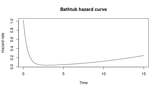

plot of chunk bathtub

Model Diagnostics

Check model fit with residual analysis:

# Fit exponential to data
fitted_exp <- dfr_exponential(lambda = coef(result))

# Cox-Snell residuals Q-Q plot
qqplot_residuals(fitted_exp, df)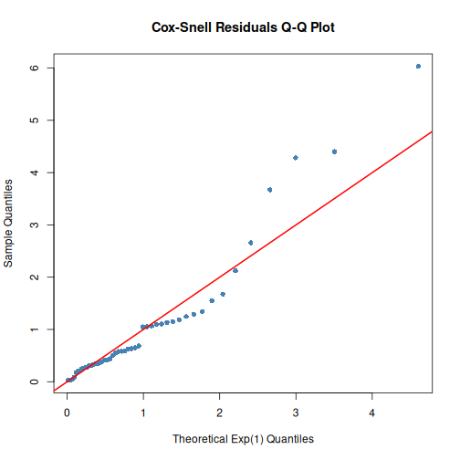

plot of chunk diagnostics

Mathematical Background

For a lifetime \(T\), the hazard function is: \[h(t) = \frac{f(t)}{S(t)}\]

From the hazard, all other quantities follow:

Function	Formula	Method
Cumulative hazard	\(H(t) = \int_0^t h(u) du\)	`cum_haz()`
Survival	\(S(t) = e^{-H(t)}\)	`surv()`
CDF	\(F(t) = 1 - S(t)\)	`cdf()`
PDF	\(f(t) = h(t) \cdot S(t)\)	`density()`

Likelihood for Survival Data

For exact observations: \(\log L = \log h(t) - H(t)\)

For right-censored: \(\log L = -H(t)\)

# Mixed data with censoring
df <- data.frame(
  t = c(1, 2, 3, 4, 5),
  delta = c(1, 1, 0, 1, 0)  # 1 = exact, 0 = censored
)

ll <- loglik(dfr_exponential())
ll(df, par = c(0.5))
#> [1] -9.579442

Documentation

Start Here:

Package Overview & Quick Start - Motivation, complete example, and quick start guide

Real-World Applications:

Reliability Engineering - Five case studies

Going Deeper:

Dynamic Failure Rate Distributions - Mathematical foundations
Creating Custom Distributions - The three-level optimization paradigm
Custom Derivatives for MLE - Analytical score and Hessian functions

Reference:

Function Reference

algebraic.dist: Generic distribution interface
likelihood.model: Likelihood model framework
algebraic.mle: MLE utilities

These binaries (installable software) and packages are in development.
They may not be fully stable and should be used with caution. We make no claims about them.
Health stats visible at Monitor.