The hardware and bandwidth for this mirror is donated by dogado GmbH, the Webhosting and Full Service-Cloud Provider. Check out our Wordpress Tutorial.
If you wish to report a bug, or if you are interested in having us mirror your free-software or open-source project, please feel free to contact us at mirror[@]dogado.de.
This repo contains numerical implementations of algorithms to estimate weighted, undirected, (possibly k-component) bipartite graphs.
finbipartite depends on the development version of spectralGraphTopology.
You can install the development version from GitHub:
> devtools::install_github("convexfi/spectralGraphTopology")
> devtools::install_github("convexfi/finbipartite")On MS Windows environments, make sure to install the most recent
version of Rtools.
library(fitHeavyTail)
library(xts)
library(quantmod)
library(igraph)
library(finbipartite)
library(readr)
set.seed(42)
# load SP500 stock prices into an xts table
stock_prices <- readRDS("examples/stocks/sp500-data-2016-2021.rds")
# number of sectors
q <- 8
# number of stocks
r <- ncol(stock_prices) - q
# total nodes in the graph
p <- r + q
colnames(stock_prices)[1:r]
#> [1] "A" "AAL" "ABBV" "ABC" "ABMD" "ABT" "ADM" "AEE" "AEP" "AES"
#> [11] "AFL" "AIG" "AIV" "AIZ" "AJG" "ALB" "ALGN" "ALK" "ALL" "ALLE"
#> [21] "ALXN" "AMCR" "AME" "AMGN" "AMP" "AMT" "ANTM" "AON" "AOS" "APA"
#> [31] "APD" "ARE" "ATO" "AVB" "AVY" "AWK" "AXP" "BA" "BAC" "BAX"
#> [41] "BDX" "BEN" "BIIB" "BIO" "BK" "BKR" "BLK" "BLL" "BMY" "BSX"
#> [51] "BXP" "C" "CAG" "CAH" "CAT" "CB" "CBOE" "CBRE" "CCI" "CE"
#> [61] "CERN" "CF" "CFG" "CHD" "CHRW" "CI" "CINF" "CL" "CLX" "CMA"
#> [71] "CME" "CMI" "CMS" "CNC" "CNP" "COF" "COG" "COO" "COP" "COST"
#> [81] "COTY" "CPB" "CPRT" "CSX" "CTAS" "CVS" "CVX" "D" "DAL" "DD"
#> [91] "DE" "DFS" "DGX" "DHR" "DLR" "DOV" "DRE" "DTE" "DUK" "DVA"
#> [101] "DVN" "DXCM" "ECL" "ED" "EFX" "EIX" "EL" "EMN" "EMR" "EOG"
#> [111] "EQIX" "EQR" "ES" "ESS" "ETN" "ETR" "EVRG" "EW" "EXC" "EXPD"
#> [121] "EXR" "FANG" "FAST" "FBHS" "FCX" "FDX" "FE" "FITB" "FLS" "FMC"
#> [131] "FRC" "FRT" "FTI" "GD" "GE" "GILD" "GIS" "GL" "GS" "GWW"
#> [141] "HAL" "HBAN" "HCA" "HES" "HFC" "HIG" "HII" "HOLX" "HON" "HRL"
#> [151] "HSIC" "HST" "HSY" "HUM" "HWM" "ICE" "IDXX" "IEX" "IFF" "ILMN"
#> [161] "INCY" "INFO" "IP" "IQV" "IRM" "ISRG" "ITW" "IVZ" "J" "JBHT"
#> [171] "JCI" "JNJ" "JPM" "K" "KEY" "KHC" "KIM" "KMB" "KMI" "KO"
#> [181] "KR" "KSU" "L" "LH" "LHX" "LIN" "LLY" "LMT" "LNC" "LNT"
#> [191] "LUV" "LYB" "MAA" "MAS" "MCK" "MCO" "MDLZ" "MDT" "MET" "MKC"
#> [201] "MKTX" "MLM" "MMC" "MMM" "MNST" "MO" "MOS" "MPC" "MRK" "MRO"
#> [211] "MS" "MSCI" "MTB" "MTD" "NDAQ" "NEE" "NEM" "NI" "NLSN" "NOC"
#> [221] "NOV" "NRG" "NSC" "NTRS" "NUE" "O" "ODFL" "OKE" "OXY" "PBCT"
#> [231] "PCAR" "PEAK" "PEG" "PEP" "PFE" "PFG" "PG" "PGR" "PH" "PKG"
#> [241] "PKI" "PLD" "PM" "PNC" "PNR" "PNW" "PPG" "PPL" "PRGO" "PRU"
#> [251] "PSA" "PSX" "PWR" "PXD" "RE" "REG" "REGN" "RF" "RHI" "RJF"
#> [261] "RMD" "ROK" "ROL" "ROP" "RSG" "RTX" "SBAC" "SCHW" "SEE" "SHW"
#> [271] "SIVB" "SJM" "SLB" "SLG" "SNA" "SO" "SPG" "SPGI" "SRE" "STE"
#> [281] "STT" "STZ" "SWK" "SYF" "SYK" "SYY" "TAP" "TDG" "TDY" "TFC"
#> [291] "TFX" "TMO" "TROW" "TRV" "TSN" "TT" "TXT" "UAL" "UDR" "UHS"
#> [301] "UNH" "UNM" "UNP" "UPS" "URI" "USB" "VAR" "VLO" "VMC" "VNO"
#> [311] "VRSK" "VRTX" "VTR" "WAB" "WAT" "WBA" "WEC" "WELL" "WFC" "WLTW"
#> [321] "WM" "WMB" "WMT" "WRB" "WST" "WY" "XEL" "XOM" "XRAY" "XYL"
#> [331] "ZBH" "ZION" "ZTS"
colnames(stock_prices)[(r+1):p]
#> [1] "XLP" "XLE" "XLF" "XLV" "XLI" "XLB" "XLRE" "XLU"
selected_sectors <- c("Consumer Staples", "Energy", "Financials",
"Health Care", "Industrials", "Materials",
"Real Estate", "Utilities")
# compute log-returns
log_returns <- diff(log(stock_prices), na.pad = FALSE)
# fit an univariate Student-t distribution to the log-returns of the market
# to obtain an estimate of the degrees of freedom (nu)
mkt_index <- Ad(getSymbols("^GSPC",
from = index(stock_prices[1]), to = index(stock_prices[nrow(stock_prices)]),
auto.assign = FALSE,
verbose = FALSE))
mkt_index_log_returns <- diff(log(mkt_index), na.pad = FALSE)
nu <- fit_mvt(mkt_index_log_returns,
nu="MLE-diag-resampled")$nu
# learn a bipartite graph with k = 8 components
graph_mrf <- learn_heavy_tail_kcomp_bipartite_graph(scale(log_returns),
r = r,
q = q,
k = 8,
nu = nu,
learning_rate = 1,
verbose = FALSE)
# save predicted labels
labels_pred <- c()
for(i in c(1:r)){
labels_pred <- c(labels_pred, which.max(graph_mrf$B[i, ]))
}
# build network
SP500 <- read_csv("examples/stocks/SP500-sectors.csv")
stock_sectors <- SP500$GICS.Sector[SP500$Symbol %in% colnames(stock_prices)[1:r]]
stock_sectors_index <- as.numeric(as.factor(stock_sectors))
net <- graph_from_adjacency_matrix(graph_mrf$adjacency, mode = "undirected", weighted = TRUE)
colors <- c("#55efc4", "#ff7675", "#0984e3", "#a29bfe", "#B33771", "#48dbfb", "#FDA7DF", "#C4E538")
V(net)$color <- c(colors[stock_sectors_index], colors)
V(net)$type <- c(rep(FALSE, r), rep(TRUE, q))
V(net)$cluster <- c(stock_sectors_index, c(1:q))
E(net)$color <- apply(as.data.frame(get.edgelist(net)), 1,
function(x) ifelse(V(net)$cluster[x[1]] == V(net)$cluster[x[2]],
colors[V(net)$cluster[x[1]]], 'grey'))
# where do our predictions differ from GICS?
mask <- labels_pred != stock_sectors_index
node_labels <- colnames(stock_prices)[1:r]
node_labels[!mask] <- NA
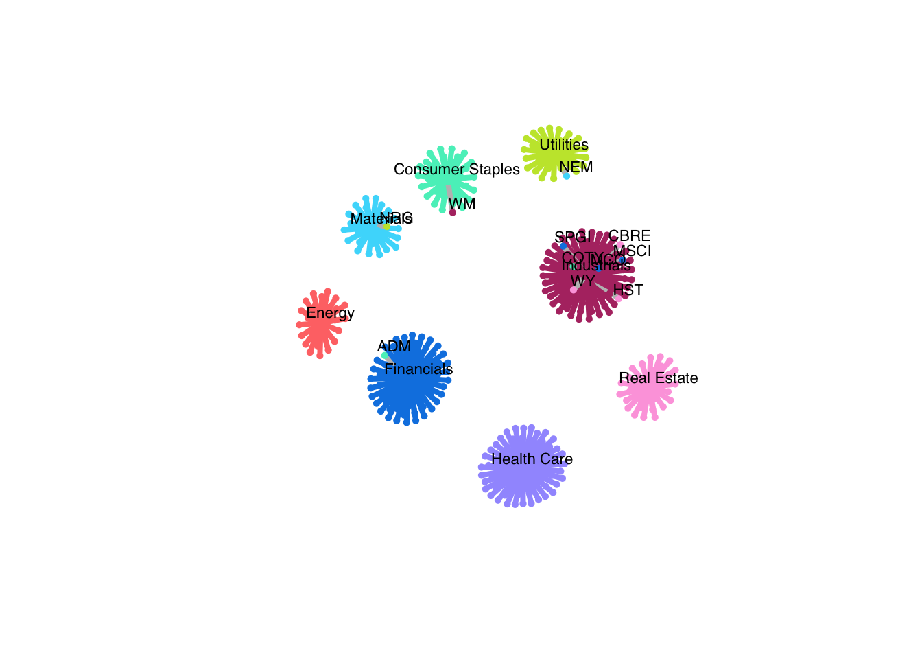
# plot network
plot(net, vertex.size = c(rep(3, r), rep(5, q)),
vertex.label = c(node_labels, selected_sectors),
vertex.label.cex = 0.7, vertex.label.dist = 1.0,
vertex.frame.color = c(colors[stock_sectors_index], colors),
layout = layout_nicely(net),
vertex.label.family = "Helvetica", vertex.label.color = "black",
vertex.shape = c(rep("circle", r), rep("square", q)),
edge.width = 4*E(net)$weight)
If you made use of this software please consider citing:
These binaries (installable software) and packages are in development.
They may not be fully stable and should be used with caution. We make no claims about them.
Health stats visible at Monitor.