The hardware and bandwidth for this mirror is donated by dogado GmbH, the Webhosting and Full Service-Cloud Provider. Check out our Wordpress Tutorial.
If you wish to report a bug, or if you are interested in having us mirror your free-software or open-source project, please feel free to contact us at mirror[@]dogado.de.
![]()
The goal of eventstream is to extract and classify events in contiguous spatio-temporal data streams of 2 or 3 dimensions. For details see (Kandanaarachchi, Hyndman, and Smith-Miles 2020).
You can install the development version of eventstream from github with:
#install.packages("devtools")
devtools::install_github("sevvandi/eventstream")This is an example of a data stream you can generate with eventstream.
library("eventstream")
library("ggplot2")
library("raster")
#> Loading required package: sp
library("maps")

str <- gen_stream(3, sd=1)
zz <- str$data
dat <- as.data.frame(t(zz))
dat.x <- 1:dim(dat)[2]
dat.y <- 1:dim(dat)[1]
mesh.xy <- eventstream:::meshgrid(dat.x,dat.y)
xyz.dat <- cbind(as.vector(mesh.xy$x), as.vector(mesh.xy$y), as.vector(as.matrix(dat)) )
xyz.dat <- as.data.frame(xyz.dat)
colnames(xyz.dat) <- c("Time", "Location", "Value")
ggplot(xyz.dat, aes(Time, Location)) + geom_raster(aes(fill=Value)) +   scale_fill_gradientn(colours=topo.colors(12)) + theme_bw()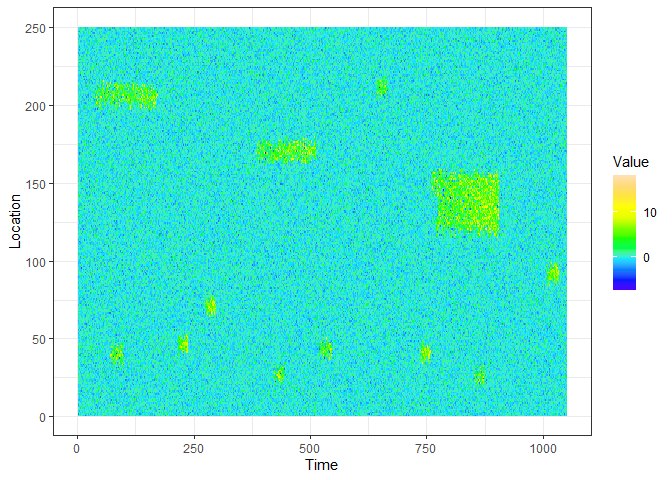
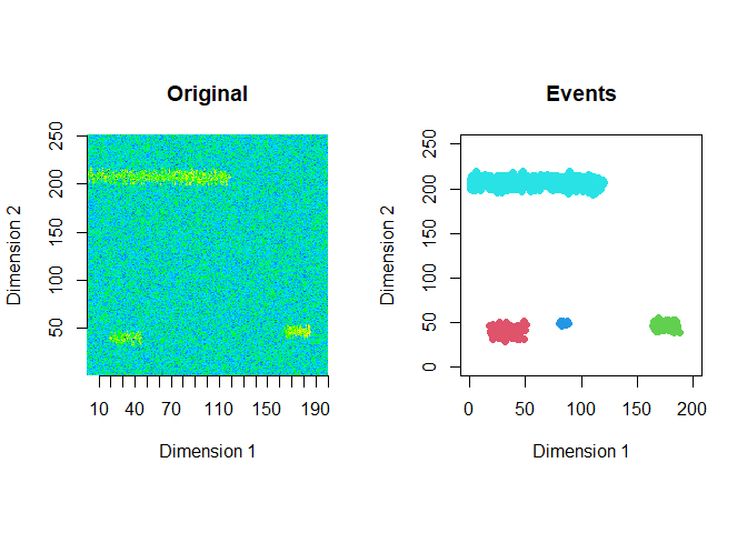
The extracted events are plotted for the first 2 windows using a window size of 200 and a step size of 50.
zz2 <- zz[1:250,]
ftrs <- extract_event_ftrs(zz2, rolling=FALSE, win_size=200, step_size = 50, vis=TRUE)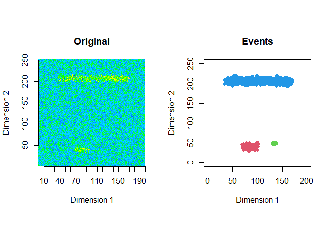
To extract 3D events we use the NO2 data from NASA’s NEO website.
data(NO2_2019)
dim(NO2_2019)
#> [1]   4 179 360
ftrs_2019 <- extract_event_ftrs(NO2_2019, thres=0.97, epsilon = 2, miniPts = 20, win_size=4, step_size=1, rolling=TRUE, tt=1, vis=FALSE)
dim(ftrs_2019)
#> [1] 17 17  4
ftrs_2019[1, , ]
#>                             [,1]          [,2]          [,3]          [,4]
#> cluster_id             2.0000000     2.0000000     2.0000000     2.0000000
#> pixels                38.0000000    76.0000000    99.0000000   110.0000000
#> length                 1.0000000     2.0000000     3.0000000     4.0000000
#> width                 10.0000000    11.0000000    11.0000000    11.0000000
#> height                 7.0000000     8.0000000     8.0000000     8.0000000
#> total_value         7441.0000000 14168.0000000 18070.0000000 19973.0000000
#> l2w_ratio              0.1000000     0.1818182     0.2727273     0.3636364
#> centroid_x             1.0000000     1.5000000     1.8484848     2.0636364
#> centroid_y            57.0263158    56.7763158    56.8080808    56.8636364
#> centroid_z            84.3684211    84.4342105    84.5555556    84.5909091
#> mean                 195.8157895   186.4210526   182.5252525   181.5727273
#> std_dev               52.8029766    43.4561122    39.9692084    39.0289140
#> slope                  0.0000000   -18.7894737   -13.0818078    -7.5821510
#> quad1                  0.0000000     0.0000000   -18.5004700   -16.9542051
#> quad2                  0.0000000     0.0000000     4.6602897    11.0686499
#> sd_from_global_mean    0.8868751     0.8927779     0.8927779     0.8927779
#> Class                  0.0000000     0.0000000     0.0000000     0.0000000
The features contain 17 events, 17 features, and 4 age brackets for the events.
First, let us visualize NO2 data for March 2019.
data(NO2_2019)
r <- raster(NO2_2019[1, ,],xmn=-179.5,xmx=179.5,ymn=-89.5,ymx=89.5,crs="+proj=longlat +datum=WGS84")
plot(r, legend=F, main="2019 March NO2 levels")
map("world",add=T, fill=FALSE, col="darkgrey")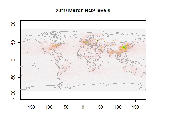
Next we extract 3D events from March - June 2019. Then we visualize 2D cross sections of these 3D events for March 2019.
data(NO2_2019)
output <- get_clusters_3d(NO2_2019, thres=0.97, epsilon = 2, miniPts = 20)
cluster.all <- output$clusters
xyz.high <- output$data
all_no2_clusters_march <- xyz.high[xyz.high[,1]==1,-1]
all_cluster_ids_march <- cluster.all$cluster[xyz.high[,1]==1]
cluster_ids_march <- all_cluster_ids_march[all_cluster_ids_march!=0]
no2_clusters_march <- all_no2_clusters_march[all_cluster_ids_march!=0,]

march_map <- matrix(0, nrow=180, ncol=360)
set.seed(123)
new_ids <- sample( length(unique(cluster_ids_march)),length(unique(cluster_ids_march)) )
new_cluster_ids <- cluster_ids_march
for(i in 1:length(unique(cluster_ids_march)) ) {
  new_cluster_ids[ cluster_ids_march== unique(cluster_ids_march)[i]] <- new_ids[i]
}

march_map[no2_clusters_march[,1:2]] <- new_cluster_ids
r <- raster(march_map,xmn=-179.5,xmx=179.5,ymn=-89.5,ymx=89.5,crs="+proj=longlat +datum=WGS84")
plot(r, legend=F)

map("world",add=T, fill=FALSE, col="darkgrey")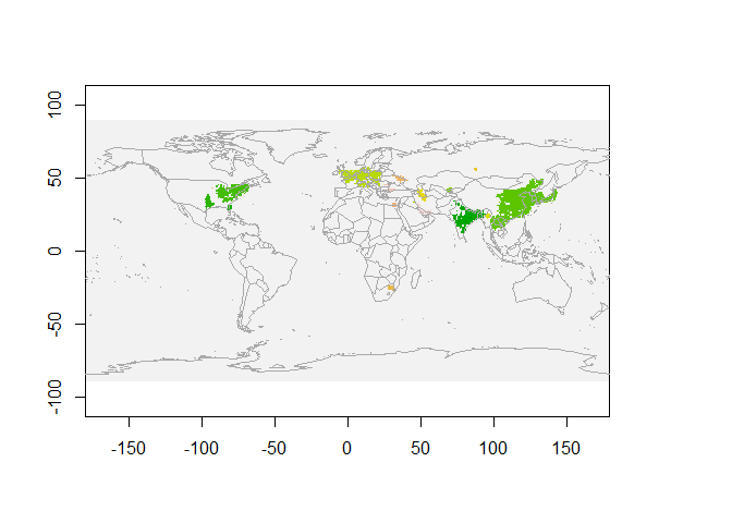
We see NO2 clusters extracted for March 2019 in the above figure. Each colour represents a single cluster.
These binaries (installable software) and packages are in development.
They may not be fully stable and should be used with caution. We make no claims about them.
Health stats visible at Monitor.