The hardware and bandwidth for this mirror is donated by dogado GmbH, the Webhosting and Full Service-Cloud Provider. Check out our Wordpress Tutorial.
If you wish to report a bug, or if you are interested in having us mirror your free-software or open-source project, please feel free to contact us at mirror[@]dogado.de.
![]()
The goal of deseats is to provide several methods to decompose seasonal time series. Among them is a new fully data-driven algorithm called DeSeaTS (deseasonalize time series) for locally weighted regression with an automatically selected bandwidth. DeSeaTS accounts for possible short-range dependence in the underlying error process. Furthermore, the base model of the BV4.1 (Berlin Procedure 4.1) can be considered as well. Permission to include the BV4.1 base model procedure was kindly provided by the Federal Statistical Office of Germany.
You can install the current version of the package from CRAN with:
install.packages("deseats")This is a basic example which shows you how to decompose a seasonal time series using the DeSeaTS algorithm:
library(deseats)

### Locally weighted regression with automatically selected bandwidth
### (here: local cubic trend)
est <- deseats(NOLABORFORCE, set_options(order_poly = 3))
est@bwidth     # The automatically selected bandwidth
#> [1] 0.2113423

### Plot of the results
plot(est, which = 1, xlab = "Year")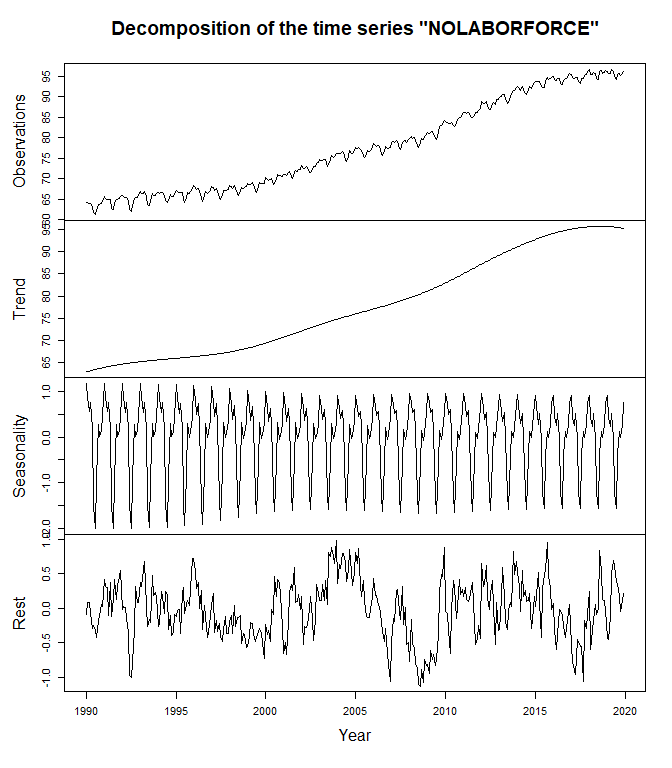
A seasonal adjustment can subsequently be easily achieved using implemented methods.
adj <- deseasonalize(est)
plot(adj, xlab = "Year", main = "The seasonally adjusted series")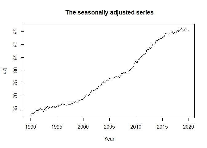
If a decomposition via the DeSeaTS algorithm is suitable, the residual series can be further analyzed using autoregressive moving-average (ARMA) models.
model <- s_semiarma(NOLABORFORCE, set_options(order_poly = 3))
model
#>
#> *******************************************
#> *                                         *
#> *        Fitted Seasonal Semi-ARMA        *
#> *                                         *
#> *******************************************
#>
#> Series: NOLABORFORCE
#>
#> Nonparametric part (Trend + Seasonality):
#> -----------------------------------------
#>
#>  Kernel:    Epanechnikov
#>  Boundary:  Shorten
#>  Bandwidth: 0.2113
#>
#>   Trend:
#>   ------
#>     Order of local polynomial: 3
#>
#>   Seasonality:
#>   ------------
#>     Frequency: 12
#>
#> Parametric part (Rest):
#> -----------------------
#>
#> Call:
#> stats::arima(x = res, order = c(ar, 0, ma), include.mean = arma_mean)
#>
#> Coefficients:
#>          ar1
#>       0.6885
#> s.e.  0.0380
#>
#> sigma^2 estimated as 0.07362:  log likelihood = -41.54,  aic = 87.08
The complete model can then be used for forecasting the seasonal time series. Forecasting intervals can be obtained either through the normality assumption or via a bootstrap.
fc <- predict(model, n.ahead = 12, method = "norm")
plot(fc, xlab = "Year", main = "A forecasting example")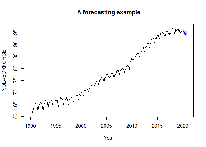
The linear locally weighted regression filters can be quickly displayed in the frequency domain.
fr <- seq(0, 0.5, 1e-04) # Frequencies
g_funs <- gain(est, lambda = fr) # Obtain correspondiong gain function values
g_deseas <- g_funs$gain_deseason # Gain function values for deseasonalization

l <- length(g_deseas[, 1])
weights_interior <- g_deseas[(l - 1) / 2 + 1, ] # middle point filter weights

plot(fr, weights_interior, type = "l", xlab = "Frequency", ylab = "Gain",
     main = "Middle point filter in the frequency domain")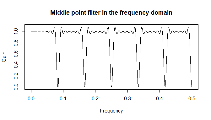
The provided decomposition methods can also be applied interactively. Run the following code.
run_decomposition()This starts a shiny app which lets you load data files, decompose the time series saved therein, and download the decomposed data.
The main functions of the package are:
deseats(): locally weighted regression with
automatically selected bandwidth for decomposition,
BV4.1(): BV4.1 base model for
decomposition,
lm_decomp(): ordinary least squares for
decomposition,
llin_decomp: local linear regression for
decomposition,
ma_decomp(): moving averages for
decomposition,
hamilton_filter(): the time series filter by
Hamilton.
The package, however, provides many other useful functions for you to discover.
The package contains several seasonal example time series from official sources.
Yuanhua Feng (Department Economics, Paderborn University, Germany) (Author)
Dominik Schulz (Department Economics, Paderborn University, Germany) (Author, Maintainer)
For questions, bug reports, etc., please contact the maintainer Mr. Dominik Schulz via dominik.schulz@uni-paderborn.de.
These binaries (installable software) and packages are in development.
They may not be fully stable and should be used with caution. We make no claims about them.
Health stats visible at Monitor.