The hardware and bandwidth for this mirror is donated by dogado GmbH, the Webhosting and Full Service-Cloud Provider. Check out our Wordpress Tutorial.
If you wish to report a bug, or if you are interested in having us mirror your free-software or open-source project, please feel free to contact us at mirror[@]dogado.de.
![]()
![]()
Diagnostic and prognostic models are typically evaluated with measures of accuracy that do not address clinical consequences. Decision-analytic techniques allow assessment of clinical outcomes but often require collection of additional information and may be cumbersome to apply to models that yield a continuous result. Decision curve analysis is a method for evaluating and comparing prediction models that incorporates clinical consequences, requires only the data set on which the models are tested, and can be applied to models that have either continuous or dichotomous results.
The dcurves package includes methods for evaluating predictive models with binary (Vickers and Elkin 2006) and time-to-event endpoints (Vickers et al. 2008). The package also includes methods for model evaluation in the case-control setting (Pfeiffer and Gail 2020).
You can install dcurves from GitHub with:
# install.packages("devtools")
devtools::install_github("ddsjoberg/dcurves")Assess models predicting binary endpoints.
library(dcurves)

dca(cancer ~ cancerpredmarker + famhistory,
    data = df_binary,
    thresholds = seq(0, 0.35, by = 0.01),
    label = list(cancerpredmarker = "Prediction Model",
                 famhistory = "Family History")) %>%
  plot(smooth = TRUE)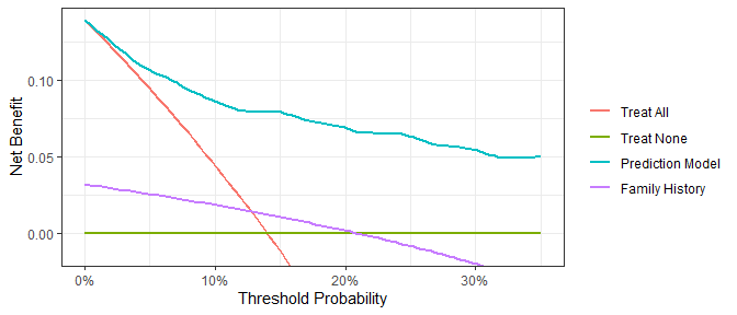
Time-to-event or survival endpoints
dca(Surv(ttcancer, cancer) ~ cancerpredmarker,
    data = df_surv,
    time = 1,
    thresholds = seq(0, 0.50, by = 0.01),
    label = list(cancerpredmarker = "Prediction Model")) %>%
  plot(smooth = TRUE)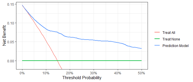
Create a customized DCA figure by first printing the ggplot code. Copy and modify the ggplot code as needed.
gg_dca <-
  dca(cancer ~ cancerpredmarker,
    data = df_binary,
    thresholds = seq(0, 0.35, by = 0.01),
    label = list(cancerpredmarker = "Prediction Model")) %>%
  plot(smooth = TRUE, show_ggplot_code = TRUE)
#> # ggplot2 code to create DCA figure -------------------------------
#> as_tibble(x) %>%
#>   dplyr::filter(!is.na(net_benefit)) %>%
#>   ggplot(aes(x = threshold, y = net_benefit, color = label)) +
#>   stat_smooth(method = "loess", se = FALSE, formula = "y ~ x",
#>     span = 0.2) +
#>   coord_cartesian(ylim = c(-0.014, 0.14)) +
#>   scale_x_continuous(labels = scales::percent_format(accuracy = 1)) +
#>   labs(x = "Threshold Probability", y = "Net Benefit", color = "") +
#> theme_bw()Pfeiffer, Ruth M, and Mitchell H Gail. (2020) “Estimating the Decision Curve and Its Precision from Three Study Designs.” Biometrical Journal 62 (3): 764–76.
Vickers, Andrew J, Angel M Cronin, Elena B Elkin, and Mithat Gonen. (2008)“Extensions to Decision Curve Analysis, a Novel Method for Evaluating Diagnostic Tests, Prediction Models and Molecular Markers.” BMC Medical Informatics and Decision Making 8 (1): 1–17.
Vickers, Andrew J, and Elena B Elkin. (2006) “Decision Curve Analysis: A Novel Method for Evaluating Prediction Models.” Medical Decision Making 26 (6): 565–74.
These binaries (installable software) and packages are in development.
They may not be fully stable and should be used with caution. We make no claims about them.
Health stats visible at Monitor.