The hardware and bandwidth for this mirror is donated by dogado GmbH, the Webhosting and Full Service-Cloud Provider. Check out our Wordpress Tutorial.
If you wish to report a bug, or if you are interested in having us mirror your free-software or open-source project, please feel free to contact us at mirror[@]dogado.de.


Country names never line up across data sources. "US",
"U.S.", "United States",
"United States of America" and "America" are
the same country, but a naïve left_join() treats them as
five. countryatlas kills that pain by making
ISO codes the universal join key and handing you a
single, ready-to-map tibble that already stitches together three
otherwise disjoint worlds:
ggplot2::map_data("world") (or Natural
Earth sf) — where countries are,The happy path is one call: world_data(2020). Everything
else is opt-in.
as_ggsql_source(),
world_query(),
interactive_map(engine = "ggsql").globe_map()), small multiples (facet_map()),
and 8 more projections (Winkel tripel, orthographic, Gall–Peters,
…).locate_country() (point-in-polygon).repair_country_names()
auto-fixes typos; country_join_all() reduce-joins many
tables at once.growth_rate(),
index_to(), share_of_world().country_borders() /
neighbors() (who borders whom),
distance_between() (great-circle distance, no
sf needed) and morans_i() (spatial
autocorrelation on the package’s own adjacency — no
spdep).dissolve_country() + the historical_codes
crosswalk resolve the USSR / Yugoslavia / Czechoslovakia to successor
states; check_country_match() now flags them (countrycode
silently maps "USSR" to Russia — caught).gini(),
theil() (population-weighted, between/within
decomposition), beta_convergence(),
sigma_convergence(), correlate_indicators(),
lag_by_country() / diff_by_country().dorling_map() and
spike_map(): two more honest displays for
totals.convert_country(to = "name_fr" / "name_es" / …).# install.packages("devtools")
devtools::install_github("PursuitOfDataScience/countryatlas")The base install is light. Heavy spatial extras (sf,
rnaturalearth, cartogram,
biscale, gganimate, leaflet, …)
live in Suggests and are only needed for the features that
use them.
| Feature / verb | Optional packages required |
|---|---|
world_map() polygon backend, spike_map(),
flow_map(), bubble_map() |
maps |
sf geometry: world_map(sf),
world_geometry(sf), locate_country(),
country_borders(), neighbors(),
morans_i() |
sf, rnaturalearth,
rnaturalearthdata |
globe_map(backend = "polygon") |
maps, mapproj |
spin_globe() (animated GIF) |
its backend’s packages, plus gifski or
magick |
bivariate_map() |
biscale, sf |
cartogram_map(), dorling_map() |
cartogram, sf |
animate_world() (animated GIF) |
gganimate (+ gifski or
magick) |
interactive_map(engine = "plotly") |
plotly |
interactive_map(engine = "ggiraph") |
ggiraph |
interactive_map(engine = "leaflet") |
leaflet, sf |
interactive_map(engine = "ggsql") |
ggsql (>= 0.4.1), duckdb,
DBI, sf |
as_ggsql_source() |
duckdb + DBI, or nanoarrow
for format = "arrow" |
simplify_geometry() |
sf; rmapshaper for the better
simplifier |
repair_country_names() /
check_country_match() with stringdist |
stringdist |
library(countryatlas)
library(ggplot2)
library(dplyr)data_2020 <- world_data(2020)
data_2020
#> # A tibble: 99,338 × 12
#> long lat group order subregion iso3c iso2c country continent region income
#> <dbl> <dbl> <dbl> <int> <chr> <chr> <chr> <chr> <chr> <chr> <fct>
#> 1 -69.9 12.5 1 1 <NA> ABW AW Aruba Americas Latin… High …
#> 2 -69.9 12.4 1 2 <NA> ABW AW Aruba Americas Latin… High …
#> 3 -69.9 12.4 1 3 <NA> ABW AW Aruba Americas Latin… High …
#> 4 -70.0 12.5 1 4 <NA> ABW AW Aruba Americas Latin… High …
#> 5 -70.1 12.5 1 5 <NA> ABW AW Aruba Americas Latin… High …
#> 6 -70.1 12.6 1 6 <NA> ABW AW Aruba Americas Latin… High …
#> 7 -70.0 12.6 1 7 <NA> ABW AW Aruba Americas Latin… High …
#> 8 -70.0 12.6 1 8 <NA> ABW AW Aruba Americas Latin… High …
#> 9 -69.9 12.5 1 9 <NA> ABW AW Aruba Americas Latin… High …
#> 10 -69.9 12.5 1 10 <NA> ABW AW Aruba Americas Latin… High …
#> # ℹ 99,328 more rows
#> # ℹ 1 more variable: gdp_per_capita <dbl>world_data() returns the map geometry, the requested
World Bank indicator(s), income and continent — already keyed on
iso3c/iso2c. Draw a choropleth with the
built-in world_map() helper (no more hand-rolled
geom_polygon() boilerplate):
world_map(data_2020, gdp_per_capita, style = "quantile",
          title = "GDP per capita, 2020")
world_map(data_2020, income, style = "categorical")
Pass one or many WDI codes with friendly names, or a year range to get a panel:
country_data(2020, c(life_exp = "SP.DYN.LE00.IN", co2 = "EN.GHG.CO2.PC.CE.AR5")) |>
  head()
#> # A tibble: 6 × 8
#>   iso3c iso2c country        continent region           income life_exp      co2
#>   <chr> <chr> <chr>          <chr>     <chr>            <fct>     <dbl>    <dbl>
#> 1 AFG   AF    Afghanistan    Asia      Middle East, No… Low i…     61.5  0.311
#> 2 ALB   AL    Albania        Europe    Europe & Centra… Upper…     77.8  1.81
#> 3 DZA   DZ    Algeria        Africa    Middle East, No… Upper…     73.3  3.90
#> 4 ASM   AS    American Samoa Oceania   East Asia & Pac… High …     72.7  0.00201
#> 5 AND   AD    Andorra        Europe    Europe & Centra… High …     79.4 NA
#> 6 AGO   AO    Angola         Africa    Sub-Saharan Afr… Lower…     63.1  0.614
Use the bundled common_indicators catalogue so you never
memorise a code, or search the full World Bank catalogue offline with
wdi_search():
head(common_indicators)
#> # A tibble: 6 × 3
#>   name                   code           description
#>   <chr>                  <chr>          <chr>
#> 1 population             SP.POP.TOTL    Population, total
#> 2 gdp                    NY.GDP.MKTP.CD GDP (current US$)
#> 3 gdp_constant           NY.GDP.MKTP.KD GDP (constant 2015 US$)
#> 4 gdp_per_capita         NY.GDP.PCAP.KD GDP per capita (constant 2015 US$)
#> 5 gdp_per_capita_current NY.GDP.PCAP.CD GDP per capita (current US$)
#> 6 gni_per_capita         NY.GNP.PCAP.CD GNI per capita (current US$)
wdi_search("renewable energy") |> head(3)
#> # A tibble: 3 × 2
#>   indicator                    name
#>   <chr>                        <chr>
#> 1 2.1_SHARE.TOTAL.RE.IN.TFEC   Renewable energy consumption(% in TFEC)
#> 2 3.1_RE.CONSUMPTION           Renewable energy consumption (TJ)
#> 3 4.1.2_REN.ELECTRICITY.OUTPUT Renewable energy electricity output (GWh)This is the headline use case. You have a frame keyed on messy
country names — join_world() standardises it and attaches
geometry in one call:
my_data <- data.frame(
  nation = c("U.S.", "S. Korea", "Czechia", "Kosovo", "Cote d'Ivoire"),
  score  = c(10, 8, 6, 4, 7)
)

my_data |>
  join_world(nation, warn = FALSE) |>
  world_map(score, title = "My data, joined on the ISO spine")
Or reconcile two messy tables directly —
"Czech Republic" vs "Czechia",
"South Korea" vs "Korea, Rep." just work:
a <- data.frame(country = c("Czechia", "South Korea"), gdp = c(1, 2))
b <- data.frame(nation  = c("Czech Republic", "Korea, Rep."), pop = c(10, 51))
country_join(a, b, country, nation)
#> # A tibble: 2 × 5
#>   country       gdp iso3c nation           pop
#>   <chr>       <dbl> <chr> <chr>          <dbl>
#> 1 Czechia         1 CZE   Czech Republic    10
#> 2 South Korea 2 KOR Korea, Rep. 51check_country_match(c("USA", "Cote d'Ivoire", "Yugoslavia", "Wakanda"))
#> # A tibble: 4 × 5
#> input iso3c matched historical suggestion
#> <chr> <chr> <lgl> <lgl> <chr>
#> 1 USA USA TRUE FALSE <NA>
#> 2 Cote d'Ivoire CIV TRUE FALSE <NA>
#> 3 Yugoslavia <NA> FALSE TRUE Yugoslavia
#> 4 Wakanda <NA> FALSE FALSE Canadaconvert_country(c("Japan", "Brazil", "Germany"), to = "flag")
#> [1] "🇯🇵" "🇧🇷" "🇩🇪"
convert_country(c("Japan", "Brazil", "Germany"), to = "currency")
#> [1] "JPY" "BRL" "EUR"
in_group(c("France", "United States", "Japan"), "EU")
#> [1] TRUE FALSE FALSEBeyond the choropleth: proportional-symbol
(bubble_map()), spikes (spike_map()),
bivariate (bivariate_map()), area-honest cartograms
(cartogram_map(), including a first-class
dorling_map()), equal-area tile grids
(tile_map()), great-circle flows (flow_map()),
an orthographic globe (globe_map()), small multiples
(facet_map()), animation (animate_world()) and
interactivity (interactive_map()).
The world as a globe, not a rectangle — with the
"polygon" backend (only maps +
mapproj, no sf) you can draw it and even
spin it:
globe_map(world_snapshot$countries, continent, backend = "polygon",
          style = "categorical", lon = 10, lat = 20)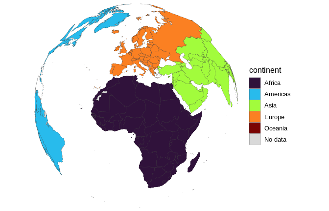
# assemble a rotating GIF (one full turn; needs gifski or magick)
spin_globe(world_snapshot$countries, continent, backend = "polygon",
           style = "categorical")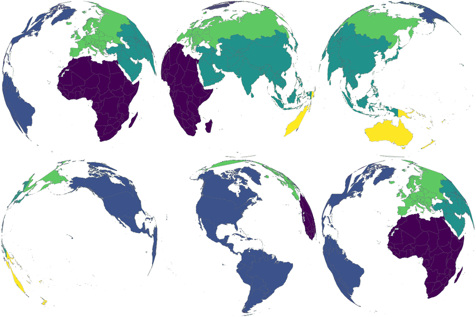
bubble_map(world_snapshot$countries, population)
ggsql draws plots in the
database (DuckDB) and returns a Vega-Lite widget — no ggplot2 or
sf runtime needed. countryatlas does the part ggsql’s
static world can’t (ISO reconciliation, overrides, the WDI join); ggsql
does the part countryatlas doesn’t (push-down + web-ready output).
world_query() emits the spatial query (no
dependencies):
world_query(gdp_per_capita, palette = "magma", transform = "log10",
            title = "GDP per capita")
#> VISUALISE gdp_per_capita AS fill
#> FROM countryatlas_world
#> DRAW spatial
#> PROJECT TO equal_earth
#> SCALE fill TO magma VIA log10
#> LABEL title => 'GDP per capita'
…and as_ggsql_source() /
interactive_map(engine = "ggsql") register your curated
table and render it in the database. See the countryatlas and
ggsql vignette.
Get point data onto the spine, repair messy names, reduce-join many
tables, and run panel analysis — all keyed on iso3c:
# normalise a total by population, so the map isn't just a population map
# (omit `pop` and SP.POP.TOTL is fetched for the relevant countries/years)
per_capita(data.frame(iso3c = c("USA", "CHN"), co2 = c(4.7e6, 1.1e7),
                      pop = c(331e6, 1412e6)), co2, pop)
#> # A tibble: 2 × 4
#>   iso3c      co2        pop co2_per_capita
#>   <chr>    <dbl>      <dbl>          <dbl>
#> 1 USA    4700000  331000000        0.0142
#> 2 CHN   11000000 1412000000        0.00779

# each country's share of a world total (within year, for a panel)
share_of_world(data.frame(iso3c = c("USA", "CHN", "IND"), co2 = c(5, 15, 3)), co2)
#> # A tibble: 3 × 3
#>   iso3c   co2 co2_share
#>   <chr> <dbl>     <dbl>
#> 1 USA       5     0.217
#> 2 CHN      15     0.652
#> 3 IND       3     0.130

# reduce-join several messy tables on the ISO spine at once
t1 <- data.frame(country = c("Czechia", "South Korea"), gdp = c(1, 2))
t2 <- data.frame(country = c("Czech Republic", "Korea, Rep."), pop = c(10, 51))
t3 <- data.frame(country = c("Czechia", "Korea"), area = c(79, 100))
country_join_all(list(t1, t2, t3), by = "country")
#> # A tibble: 2 × 7
#>   country.x     gdp iso3c country.y        pop country  area
#>   <chr>       <dbl> <chr> <chr>          <dbl> <chr>   <dbl>
#> 1 Czechia         1 CZE   Czech Republic    10 Czechia    79
#> 2 South Korea     2 KOR   Korea, Rep.       51 Korea     100

# great-circle distance between two countries' centroids (no sf needed)
distance_between("France", "Germany")
#> [1] 802.3524Dissolved entities poison country joins twice over: most are silently
dropped, and some are silently mismatched — countrycode
resolves "USSR" to Russia alone, so Soviet-era totals
quietly become Russian totals. check_country_match() flags
both cases, and dissolve_country() resolves them to
successor states (one-to-many, dated) via the curated
historical_codes crosswalk:
check_country_match(c("USSR", "Yugoslavia", "France"))
#> # A tibble: 3 × 5
#>   input      iso3c matched historical suggestion
#>   <chr>      <chr> <lgl>   <lgl>      <chr>
#> 1 USSR       RUS   TRUE    TRUE       <NA>
#> 2 Yugoslavia <NA>  FALSE   TRUE       Yugoslavia
#> 3 France     FRA   TRUE    FALSE      <NA>
dissolve_country("Czechoslovakia")
#> # A tibble: 2 × 5
#>   input          historical     dissolved iso3c country
#>   <chr>          <chr>              <int> <chr> <chr>
#> 1 Czechoslovakia Czechoslovakia      1993 CZE   Czechia
#> 2 Czechoslovakia Czechoslovakia 1993 SVK SlovakiaWorld inequality between people, not country units — and how much of it sits between continents vs within them:
snap <- world_snapshot$countries
gini(snap$gdp_per_capita, weights = snap$population)
#> [1] 0.6094909
theil(snap$gdp_per_capita, weights = snap$population, groups = snap$continent)
#> # A tibble: 3 × 3
#>   component value share
#>   <chr>     <dbl> <dbl>
#> 1 total     0.678 1
#> 2 between   0.310 0.458
#> 3 within    0.368 0.542
beta_convergence() / sigma_convergence()
test whether poor countries are catching up;
correlate_indicators() screens indicator pairs
(pairwise-complete, with n reported); and
morans_i() measures spatial autocorrelation on the
package’s own border adjacency — no spdep required.
repair_country_names() auto-fixes typos to the closest
known country, locate_country(lon, lat) tags coordinates
with the country that contains them, neighbors() /
country_borders() answer “who shares a border with whom”,
growth_rate() / index_to() /
complete_years() add panel metrics and fill panel gaps, and
country_codes() exposes the whole countrycode crosswalk as
a tidy, pipeable lookup.
The bundled world_snapshot (a curated indicator set for
one recent year, plus metadata) means examples, tests and vignettes all
run without the World Bank API.
See the vignettes — Getting started, Joining your own data, Modern maps with sf & projections, Beyond the choropleth, and countryatlas and ggsql — and the reference site.
These binaries (installable software) and packages are in development.
They may not be fully stable and should be used with caution. We make no claims about them.
Health stats visible at Monitor.