The hardware and bandwidth for this mirror is donated by dogado GmbH, the Webhosting and Full Service-Cloud Provider. Check out our Wordpress Tutorial.
If you wish to report a bug, or if you are interested in having us mirror your free-software or open-source project, please feel free to contact us at mirror[@]dogado.de.

colors3d

This R package provides functions to help generate two-dimensional and three-dimensional color gradient legends.

The three main functions, colors3d, colors2d, and colorwheel2d generate a color for each row of a user-supplied data set with 2-3 columns. These can then be used for plotting in various ways.

Installation

You can install colors3d from GitHub with devtools::install_github("matthewkling/colors3d") or from CRAN with install.packages("colors3d").

Examples

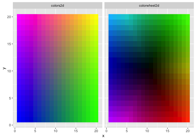
Here’s a simple application of the three color mapping functions. This example uses tidyverse, but this would all work in base R as well:

library(colors3d)
library(tidyverse)

# simulate a 3D data set
d <- expand_grid(x = 1:20, y = 1:20, z = 1:4)

# define and plot some 2D color mappings
d$colors2d <- colors2d(d[, 1:2])
d$colorwheel2d <- colorwheel2d(d[, 1:2])
d %>%
      gather(mapping, color, colors2d, colorwheel2d) %>%
      ggplot(aes(x, y, fill = color)) +
      facet_wrap(~mapping) +
      geom_raster() +
      scale_fill_identity()

# define and plot a 3D color mapping
d$color3d <- colors3d(d[, 1:3])
d %>%
      ggplot(aes(x, y, fill = color3d)) +
      facet_wrap(~z, nrow = 1, labeller = label_both) +
      geom_raster() +
      scale_fill_identity()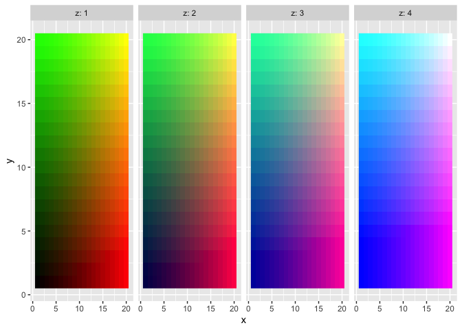

In a more realistic application, we often want to create a pair of plots for a given visualization: a “legend” in which the x and y dimensions match those used to create the color mapping, and a second plot in which the colors are then displayed in a different data space. This allows users to understand relationships among four dimensions of the data (or 5, if a 3D color mapping is used). Let’s use the storms dataset (from dplyr) as an example, with hurricane windspeed, size, longitude, and latitude as our variables of interest:

d <- na.omit(storms)
d$color <- colors2d(select(d, wind, hurricane_force_diameter),
                    xtrans = "rank", ytrans = "rank")

p1 <- ggplot(d, aes(wind, hurricane_force_diameter, color = color)) +
      geom_point() +
      scale_color_identity()
p2 <- ggplot() +
      geom_polygon(data = map_data("state"), 
                   aes(long, lat, group = group)) +
      geom_path(data = d, 
                aes(long, lat, color = color,
                    group = paste(name, year))) +
      scale_color_identity() +
      coord_cartesian(xlim = range(d$long),
                      ylim = range(d$lat))

library(patchwork)
p1 + p2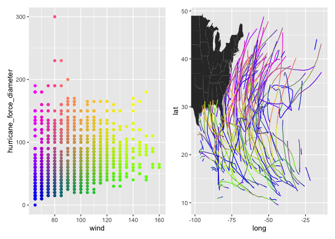

These binaries (installable software) and packages are in development.
They may not be fully stable and should be used with caution. We make no claims about them.
Health stats visible at Monitor.