The hardware and bandwidth for this mirror is donated by dogado GmbH, the Webhosting and Full Service-Cloud Provider. Check out our Wordpress Tutorial.
If you wish to report a bug, or if you are interested in having us mirror your free-software or open-source project, please feel free to contact us at mirror[@]dogado.de.

cograph

cograph is a modern R package for the analysis, visualization, and manipulation of complex networks. It provides publication-ready plotting with customizable layouts, node shapes, edge styles, and themes through an intuitive, pipe-friendly API. First-class support for Transition Network Analysis (TNA), multilayer networks, and community detection.

Installation

# Install from CRAN
install.packages("cograph")

# Development version from GitHub
devtools::install_github("sonsoleslp/cograph")

Features

Network Plotting

Function	Description
`splot()`	Base R network plot (core engine)
`soplot()`	Grid/ggplot2 network rendering
`tplot()`	qgraph drop-in replacement for TNA
`plot_htna()`	Hierarchical multi-group TNA layouts
`plot_mtna()`	Multi-cluster TNA with shape containers
`plot_mcml()`	Markov Chain Multi-Level visualization
`plot_mlna()`	Multilayer 3D perspective networks
`plot_mixed_network()`	Combined symmetric/asymmetric edges

Flow and Comparison Plots

Function	Description
`plot_transitions()`	Alluvial/Sankey flow diagrams
`plot_alluvial()`	Alluvial wrapper with flow coloring
`plot_trajectories()`	Individual tracking with line bundling
`plot_chord()`	Chord diagrams with ticks
`plot_heatmap()`	Adjacency heatmaps with clustering
`plot_compare()`	Difference network visualization
`plot_bootstrap()`	Bootstrap CI result plots
`plot_permutation()`	Permutation test result plots

Community and Higher-Order Structure

Function	Description
`overlay_communities()`	Community blob overlays on network plots
`plot_simplicial()`	Higher-order pathway (simplicial complex) visualization
`detect_communities()`	11 igraph algorithms with shorthand wrappers
`communities()`	Unified community detection interface

Network Analysis

Function	Description
`centrality()`	23+ centrality measures with individual wrappers
`motifs()` / `subgraphs()`	Motif/triad census with per-actor windowing
`robustness()`	Network robustness analysis
`disparity_filter()`	Backbone extraction (Serrano et al. 2009)
`cluster_summary()`	Between/within cluster weight aggregation
`build_mcml()`	Markov Chain Multi-Level model construction
`summarize_network()`	Comprehensive network-level statistics
`verify_with_igraph()`	Cross-validation against igraph
`simplify()`	Prune weak edges

Multilayer Networks

Function	Description
`supra_adjacency()`	Supra-adjacency matrix construction
`layer_similarity()`	Layer comparison measures
`aggregate_layers()`	Weight aggregation across layers
`plot_ml_heatmap()`	Multilayer heatmaps with 3D perspective

Examples

TNA Plot

The primary use case: visualize transition networks from the tna package.

library(tna)
library(cograph)

# Build a TNA model from sequence data
fit <- tna(engagement)

# One-liner visualization
splot(fit)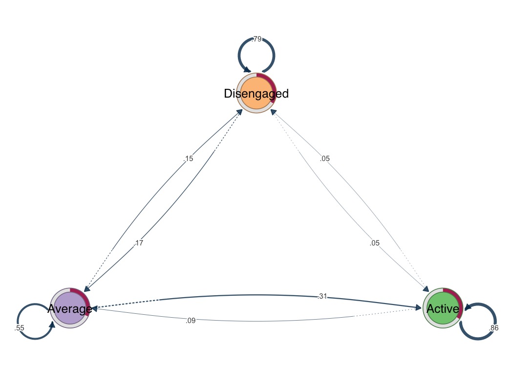

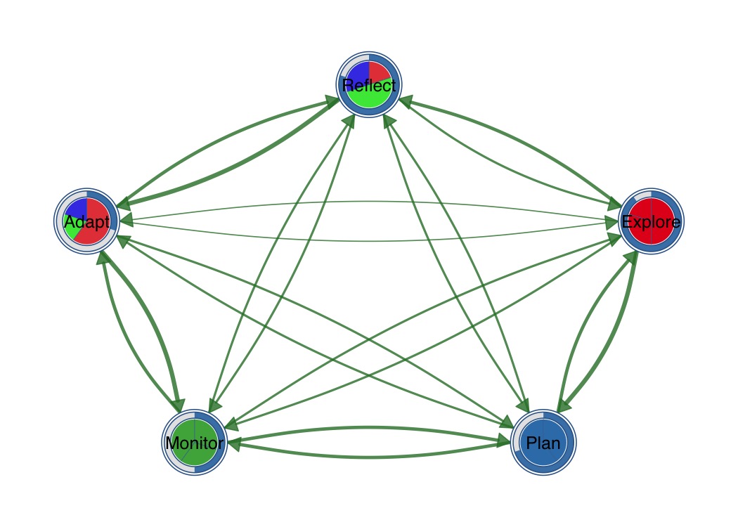
Simple Network

library(cograph)

# Create a transition matrix
states <- c("Explore", "Plan", "Monitor", "Adapt", "Reflect")
mat <- matrix(
  c(0.0, 0.4, 0.2, 0.1, 0.3,
    0.3, 0.0, 0.3, 0.2, 0.2,
    0.2, 0.3, 0.0, 0.3, 0.2,
    0.1, 0.2, 0.4, 0.0, 0.3,
    0.2, 0.2, 0.2, 0.4, 0.0),
  nrow = 5, byrow = TRUE,
  dimnames = list(states, states)
)

splot(mat)

Layouts

par(mfrow = c(2, 2), mar = c(1, 1, 2, 1))
splot(mat, layout = "oval",   title = "oval")
splot(mat, layout = "circle", title = "circle")
splot(mat, layout = "kk",     title = "kk")
splot(mat, layout = "fr",     title = "fr")

Edge Styling

splot(mat,
  curvature = 0.3,
  arrow_size = 0.02,
  edge_width = 3
)

Node Shapes

shapes <- c("circle", "square", "hexagon", "diamond", "triangle")

splot(mat,
  node_shape = shapes,
  node_fill = c("#E63946", "#457B9D", "#2A9D8F", "#E9C46A", "#F4A261"),
  layout = "circle"
)

Donuts

Donut nodes show proportional fill with optional polygon shapes.

fills <- c(0.9, 0.7, 0.5, 0.3, 0.8)

splot(mat,
  donut_fill = fills,
  donut_color = "steelblue",
  donut_shape = c("circle", "hexagon", "square", "diamond", "triangle")
)

Pies

Pie chart nodes with per-node color palettes.

pie_vals <- list(
  c(0.5, 0.3, 0.2),
  c(0.4, 0.4, 0.2),
  c(0.3, 0.3, 0.4),
  c(0.6, 0.2, 0.2),
  c(0.2, 0.5, 0.3)
)

pie_cols <- list(
  c("#E63946", "#457B9D", "#2A9D8F"),
  c("#264653", "#E9C46A", "#F4A261"),
  c("#F72585", "#7209B7", "#3A0CA3"),
  c("#003049", "#D62828", "#F77F00"),
  c("#606C38", "#283618", "#DDA15E")
)

splot(mat,
  node_shape = "pie",
  pie_values = pie_vals,
  pie_colors = pie_cols,
  layout = "circle"
)

Donut + Pie Combo

Combine outer donut ring with inner pie segments.

splot(mat,
  donut_fill = fills,
  donut_color = "steelblue",
  pie_values = pie_vals,
  pie_colors = c("#E41A1C", "#377EB8", "#4DAF4A")
)

Chord Diagram

plot_chord(mat, title = "Transition Chord Diagram")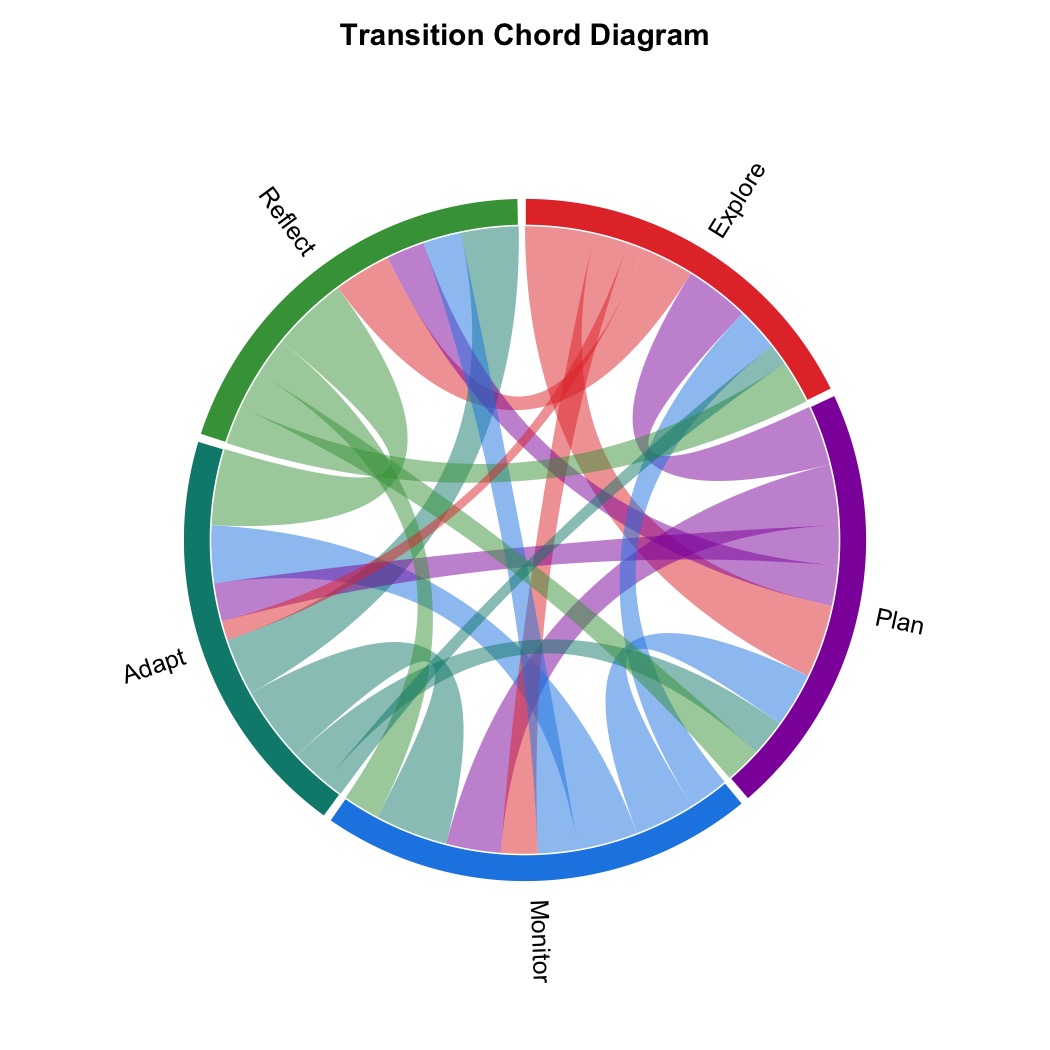

Heatmap

plot_heatmap(mat, show_values = TRUE, colors = "viridis",
             value_fontface = "bold", title = "Transition Heatmap")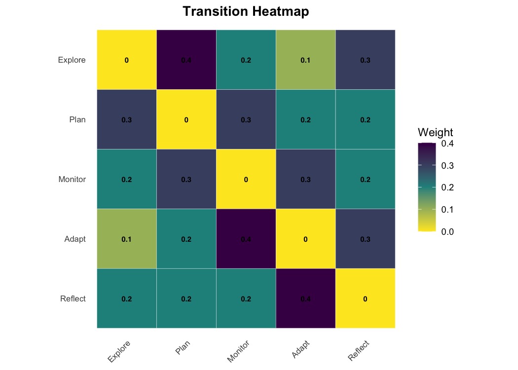

Alluvial Flow

plot_transitions(mat, flow_color_by = "from", flow_alpha = 0.5,
                 from_title = "Source", to_title = "Target")

License

MIT License.

These binaries (installable software) and packages are in development.
They may not be fully stable and should be used with caution. We make no claims about them.
Health stats visible at Monitor.