
The hardware and bandwidth for this mirror is donated by dogado GmbH, the Webhosting and Full Service-Cloud Provider. Check out our Wordpress Tutorial.
If you wish to report a bug, or if you are interested in having us mirror your free-software or open-source project, please feel free to contact us at mirror[@]dogado.de.
![]()
Cognostics are univariate statistics (or metrics) for a subset of
data. When paired with the underlying data of visualizations, cognostics
are a powerful tool for ordering and filtering the visualizations.
add_panel_cogs() will automatically append cognostics for
each plot player in a given panel column. The newly appended data can be
fed into a trelliscopejs widget
for easy viewing.
You can install autocogs from github with:
pak::pak("schloerke/autocogs")library(autocogs)
library(tidyverse)
#> ── Attaching packages ─────────────────────────────────────── tidyverse 1.3.0 ──
#> ✔ ggplot2 3.3.3.9000 ✔ purrr 0.3.4
#> ✔ tibble 3.1.1 ✔ dplyr 1.0.5
#> ✔ tidyr 1.1.3 ✔ stringr 1.4.0
#> ✔ readr 1.4.0 ✔ forcats 0.5.1
#> ── Conflicts ────────────────────────────────────────── tidyverse_conflicts() ──
#> ✖ dplyr::filter() masks stats::filter()
#> ✖ dplyr::lag() masks stats::lag()
library(gapminder)
# remotes::install_github("hafen/trelliscopejs")
# remotes::install_github("schloerke/trelliscopejs@autocogs")
library(trelliscopejs)
# Explore
p <-
ggplot(gapminder, aes(year, lifeExp)) +
geom_line(aes(group = country)) +
geom_smooth(method = "lm", formula = y ~ x)
p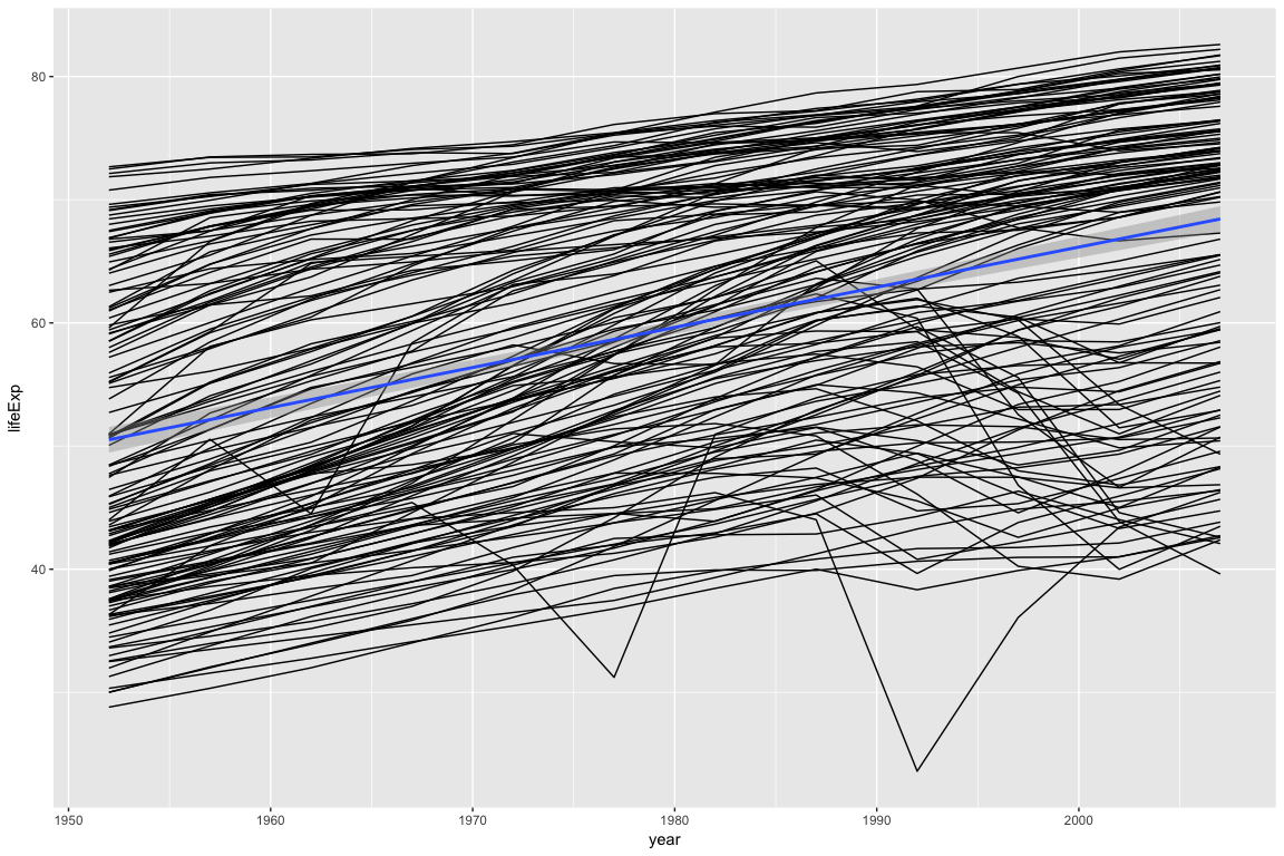
Looking at the plot above, most countries follow a linear trend: As the year increases, life expectancy goes up. A few countries do not follow a linear trend.
In the examples below, we will extract cognostics to aid in exploring the countries whose life expectancy is not linear.
trelliscopejs::facet_trelliscope()ggplot(gapminder, aes(year, lifeExp)) +
geom_smooth(method = "lm", formula = y ~ x) +
geom_line() +
trelliscopejs::facet_trelliscope(
~ country + continent,
nrow = 3, ncol = 6,
self_contained = TRUE,
auto_cog = TRUE,
state = list(
# set the state to display the country, continent, and R^2 value
# sorted by ascending R^2 value
sort = list(trelliscopejs::sort_spec("_lm_r2")),
labels = c("country", "continent", "_lm_r2")
),
path = "readme-figs/facet"
)
#> using data from the first layer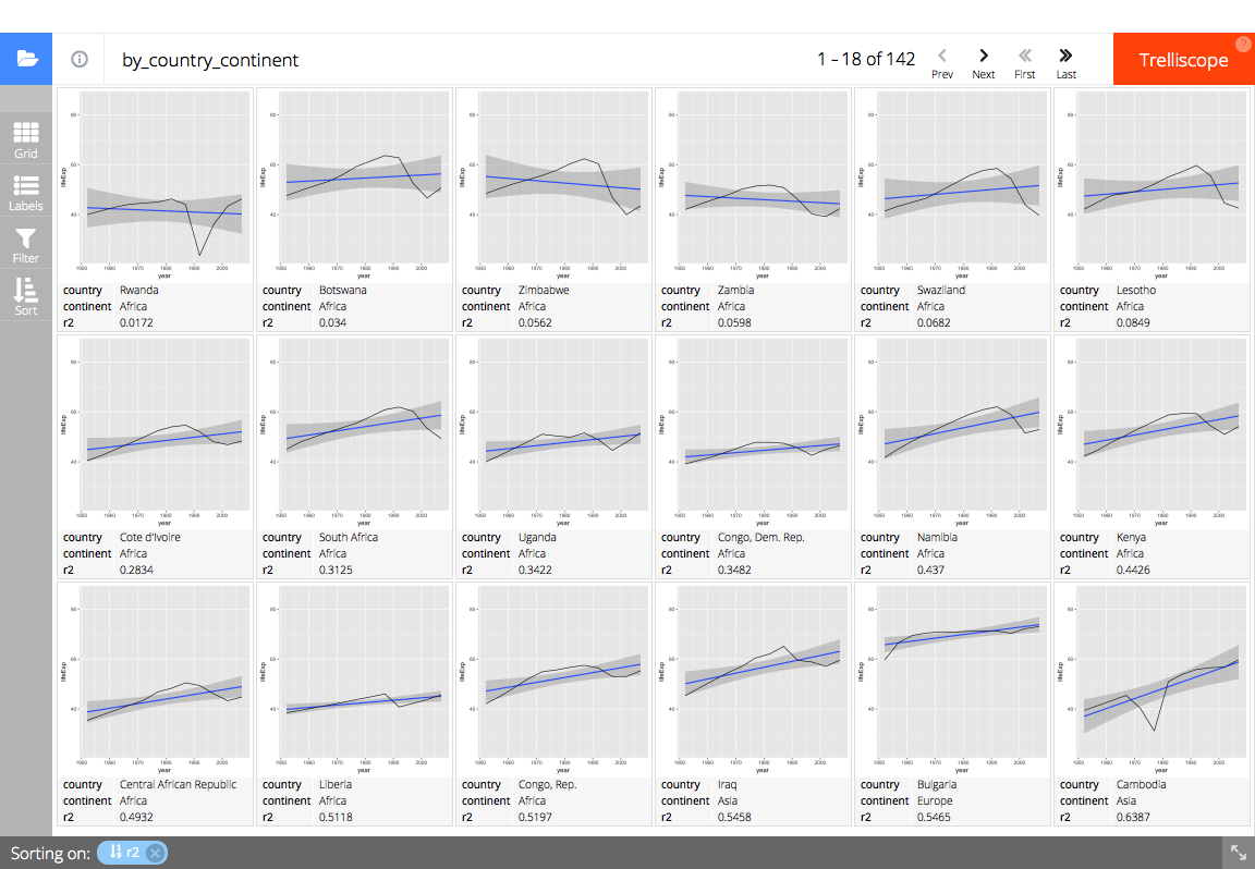
# (screen shot of trelliscopejs widget)trelliscopejs::trelliscope()This is a full, start to finish example how automatic cognostics could be inserted into a data exploration workflow.
# Find a consistent y range
y_range <- range(gapminder$lifeExp)

## # Set up data and panel column
gapminder %>%
  group_by(country, continent) %>%
  # nest the data according to the country and continent
  nest() %>%
  mutate(
    # create a column of plots with a
    # * line
    # * linear model
    panel = lapply(data, function(dt) {
      ggplot(dt, aes(year, lifeExp)) +
        geom_smooth(method = "lm", formula = y ~ x) +
        geom_line() +
        ylim(y_range[1], y_range[2])
    })
  ) %>%
  print() ->
gap_data
#> # A tibble: 142 x 4
#> # Groups:   country, continent [142]
#>    country     continent data                  panel
#>    <fct>       <fct>     <list>                <list>
#>  1 Afghanistan Asia      <tibble[,4] [12 × 4]> <gg>
#>  2 Albania     Europe    <tibble[,4] [12 × 4]> <gg>
#>  3 Algeria     Africa    <tibble[,4] [12 × 4]> <gg>
#>  4 Angola      Africa    <tibble[,4] [12 × 4]> <gg>
#>  5 Argentina   Americas  <tibble[,4] [12 × 4]> <gg>
#>  6 Australia   Oceania   <tibble[,4] [12 × 4]> <gg>
#>  7 Austria     Europe    <tibble[,4] [12 × 4]> <gg>
#>  8 Bahrain     Asia      <tibble[,4] [12 × 4]> <gg>
#>  9 Bangladesh  Asia      <tibble[,4] [12 × 4]> <gg>
#> 10 Belgium     Europe    <tibble[,4] [12 × 4]> <gg>
#> # … with 132 more rows

# Double check the plot worked...
# Look at the first panel (ggplot2 plot) of Afghanistan
gap_data$panel[[1]]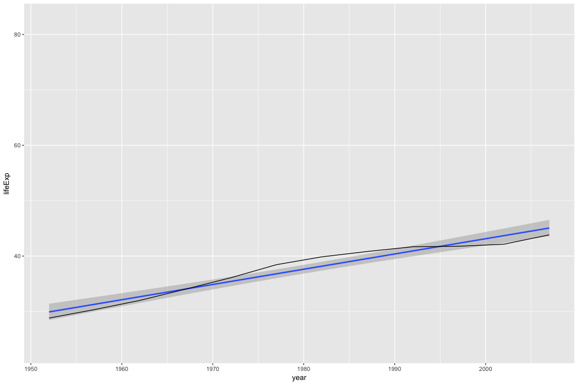
#!!!!!!!!!!
# Add cognostic information given the panel column plots
#!!!!!!!!!!
gap_data %>%
  autocogs::add_panel_cogs() %>%
  ungroup() %>%
  # double check it was added
  print(width = 100) ->
full_gap_data
#> # A tibble: 142 x 10
#>    country     continent data                  panel  `_smooth`
#>    <fct>       <fct>     <list>                <list> <list>
#>  1 Afghanistan Asia      <tibble[,4] [12 × 4]> <gg>   <tibble[,3] [1 × 3]>
#>  2 Albania     Europe    <tibble[,4] [12 × 4]> <gg>   <tibble[,3] [1 × 3]>
#>  3 Algeria     Africa    <tibble[,4] [12 × 4]> <gg>   <tibble[,3] [1 × 3]>
#>  4 Angola      Africa    <tibble[,4] [12 × 4]> <gg>   <tibble[,3] [1 × 3]>
#>  5 Argentina   Americas  <tibble[,4] [12 × 4]> <gg>   <tibble[,3] [1 × 3]>
#>  6 Australia   Oceania   <tibble[,4] [12 × 4]> <gg>   <tibble[,3] [1 × 3]>
#>  7 Austria     Europe    <tibble[,4] [12 × 4]> <gg>   <tibble[,3] [1 × 3]>
#>  8 Bahrain     Asia      <tibble[,4] [12 × 4]> <gg>   <tibble[,3] [1 × 3]>
#>  9 Bangladesh  Asia      <tibble[,4] [12 × 4]> <gg>   <tibble[,3] [1 × 3]>
#> 10 Belgium     Europe    <tibble[,4] [12 × 4]> <gg>   <tibble[,3] [1 × 3]>
#>    `_lm`            `_x`           `_y`           `_bivar`        `_n`
#>    <list>           <list>         <list>         <list>          <list>
#>  1 <tibble[,19] [1… <tibble[,5] [… <tibble[,5] [… <tibble[,2] [1… <tibble[,5] […
#>  2 <tibble[,19] [1… <tibble[,5] [… <tibble[,5] [… <tibble[,2] [1… <tibble[,5] […
#>  3 <tibble[,19] [1… <tibble[,5] [… <tibble[,5] [… <tibble[,2] [1… <tibble[,5] […
#>  4 <tibble[,19] [1… <tibble[,5] [… <tibble[,5] [… <tibble[,2] [1… <tibble[,5] […
#>  5 <tibble[,19] [1… <tibble[,5] [… <tibble[,5] [… <tibble[,2] [1… <tibble[,5] […
#>  6 <tibble[,19] [1… <tibble[,5] [… <tibble[,5] [… <tibble[,2] [1… <tibble[,5] […
#>  7 <tibble[,19] [1… <tibble[,5] [… <tibble[,5] [… <tibble[,2] [1… <tibble[,5] […
#>  8 <tibble[,19] [1… <tibble[,5] [… <tibble[,5] [… <tibble[,2] [1… <tibble[,5] […
#>  9 <tibble[,19] [1… <tibble[,5] [… <tibble[,5] [… <tibble[,2] [1… <tibble[,5] […
#> 10 <tibble[,19] [1… <tibble[,5] [… <tibble[,5] [… <tibble[,2] [1… <tibble[,5] […
#> # … with 132 more rows

# Display the panel and cognostics in a trelliscopejs widget
trelliscopejs::trelliscope(
  full_gap_data, "gapminder life expectancy",
  panel_col = "panel",
  ncol = 6, nrow = 3,
  auto_cog = FALSE,
  self_contained = TRUE,
  state = list(
    # sort by ascending R^2 value (percent explained by linear model)
    sort = list(trelliscopejs::sort_spec("_lm_r2")),
    # display the country, continent, and R^2 value
    labels = c("country", "continent", "_lm_r2")
  ),
  path = "readme-figs/manually"
)
#> New names:
#> * min -> min...26
#> * max -> max...27
#> * mean -> mean...28
#> * median -> median...29
#> * var -> var...30
#> * ...
#> Warning: Removed 4 rows containing missing values (geom_smooth).
#> Warning: Removed 8 rows containing missing values (geom_smooth).
# (screen shot of trelliscopejs widget)add_cog_group() to add a custom cognostics group.add_layer_cogs() to call which cognostics groups should
be executed for a given plot layer.Using existing code from the autocogs package, we will
add the univariate continuous cognostics group.
add_cog_group(
  "univariate_continuous",
  field_info("x", "continuous"),
  "univariate metrics for continuous data",
  function(x, ...) {
    x_range <- range(x, na.rm = TRUE)
    list(
      min = cog_desc(x_range[1], "minimum of non NA data"),
      max = cog_desc(x_range[2], "maximum of non NA data"),
      mean = cog_desc(mean(x, na.rm = TRUE), "mean of non NA data"),
      median = cog_desc(median(x, na.rm = TRUE), "median of non NA data"),
      var = cog_desc(var(x, na.rm = TRUE), "variance of non NA data")
    )
  }
)
We can then call the 'univariate_continuous' cognostics
group whenever a geom_rug layer is added in a ggplot2 plot
object using the code below.
add_layer_cogs(
  # load_all(); p <- qplot(x = 1, y = Sepal.Length, data = iris, geom = "boxplot"); plot_cogs(p)
  "geom_boxplot",
  "boxplot plot",
  cog_group_df(
    "univariate_continuous", "y", "_y",
    "boxplot", "y", "_boxplot",
    "univariate_counts", "y", "_n"
  )
)
These binaries (installable software) and packages are in development.
They may not be fully stable and should be used with caution. We make no claims about them.
Health stats visible at Monitor.