The hardware and bandwidth for this mirror is donated by dogado GmbH, the Webhosting and Full Service-Cloud Provider. Check out our Wordpress Tutorial.
If you wish to report a bug, or if you are interested in having us mirror your free-software or open-source project, please feel free to contact us at mirror[@]dogado.de.
The First-order Integer-valued Autoregressive (INAR(1)) model with zero-inflated (ZI-INAR(1)) and hurdle (H-INAR(1)) innovations is widely used in studying integer-valued time-series data, such as crime count and heatwave frequency. This work implemented the INAR(1) models in Stan.
You can install ZIHINAR1 from GitHub with:
remotes::install_github("fushengyy/ZIHINAR1")Or you can install the released version of ZIHINAR1 from CRAN with:
install.packages("ZIHINAR1")The package contains main function named get_stanfit().
stan_fit <- get_stanfit(mod_type, distri, y, n_pred = 4,
                        thin = 2, chains = 1, iter = 2000, warmup = iter/2,
seed = NA)mod_type: Character string indicating the model
type. Use "zi" for zero-inflated models and
"h" for hurdle models.
distri: Innovation distribution. Options:
"poi": Poisson
"nb": Negative Binomial
"gp": Generalized Poisson (ZI only)
y: A numeric vector of integers representing the
observed data.
n_pred: Integer specifying the number of time points
for future predictions (default is 4).
thin: Integer indicating the thinning interval for
Stan sampling (default is 2).
chains: Integer specifying the number of Markov
chains to run (default is 1).
iter: Integer specifying the total number of
iterations per chain (default is 2000).
warmup: Integer specifying the number of warmup
iterations per chain (default is iter/2).
seed: Numeric seed for reproducibility (default is
NA).
The following are examples showing how to fit the INAR(1) model when data is generated from a zero-inflated Negative Binomial (ZINB) distribution.
library(ZIHINAR1)
y_data <- data_simu(n = 100, alpha = 0.5, rho = 0.3, lambda = 5, disp = 2,
mod_type = "zi", distri = "nb")
stan_fit <- get_stanfit(mod_type = "zi", distri = "nb", y = y_data, n_pred = 5,
iter = 2000, chains = 1, warmup = 500,
thin = 2, seed = 42)
#>
#> SAMPLING FOR MODEL 'anon_model' NOW (CHAIN 1).
#> Chain 1:
#> Chain 1: Gradient evaluation took 0.000715 seconds
#> Chain 1: 1000 transitions using 10 leapfrog steps per transition would take 7.15 seconds.
#> Chain 1: Adjust your expectations accordingly!
#> Chain 1:
#> Chain 1:
#> Chain 1: Iteration: 1 / 2000 [ 0%] (Warmup)
#> Chain 1: Iteration: 200 / 2000 [ 10%] (Warmup)
#> Chain 1: Iteration: 400 / 2000 [ 20%] (Warmup)
#> Chain 1: Iteration: 501 / 2000 [ 25%] (Sampling)
#> Chain 1: Iteration: 700 / 2000 [ 35%] (Sampling)
#> Chain 1: Iteration: 900 / 2000 [ 45%] (Sampling)
#> Chain 1: Iteration: 1100 / 2000 [ 55%] (Sampling)
#> Chain 1: Iteration: 1300 / 2000 [ 65%] (Sampling)
#> Chain 1: Iteration: 1500 / 2000 [ 75%] (Sampling)
#> Chain 1: Iteration: 1700 / 2000 [ 85%] (Sampling)
#> Chain 1: Iteration: 1900 / 2000 [ 95%] (Sampling)
#> Chain 1: Iteration: 2000 / 2000 [100%] (Sampling)
#> Chain 1:
#> Chain 1: Elapsed Time: 3.277 seconds (Warm-up)
#> Chain 1: 9.208 seconds (Sampling)
#> Chain 1: 12.485 seconds (Total)
#> Chain 1:
get_est(distri = "nb", stan_fit = stan_fit)
#> Mean SD Median Q2.5 Q97.5 Rhat
#> alpha 0.5307909 0.04108348 0.5327549 0.44979898 0.6019402 1.0047284
#> rho 0.3696123 0.12017678 0.3837477 0.07870574 0.5645864 1.0047853
#> lambda 4.9954050 0.82387796 5.0098591 3.52989514 6.5890245 0.9998295
#> phi 2.4923431 1.50853128 2.1013737 0.70294059 6.5018753 0.9997752
#> 95%_HPD_Lower 95%_HPD_Upper
#> alpha 0.45032117 0.6028335
#> rho 0.08011943 0.5648035
#> lambda 3.64535329 6.6350831
#> phi 0.48503911 5.3722200
get_mod_sel(y = y_data, mod_type = "zi", distri = "nb", stan_fit = stan_fit)
#> EAIC EBIC DIC WAIC1 WAIC2
#> 1 519.2344 529.6149 527.1945 514.9319 515.2939
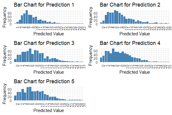
get_pred(stan_fit = stan_fit)
#> $summary
#> Mode Median IQR Min Max
#> y_pred.1 5 7 5 1 39
#> y_pred.2 3 6 7 0 30
#> y_pred.3 4 6 7 0 32
#> y_pred.4 6 6 6 0 28
#> y_pred.5 2 6 7 0 40
#>
#> $plots
#> $plots[[1]]
#>
#> $plots[[2]]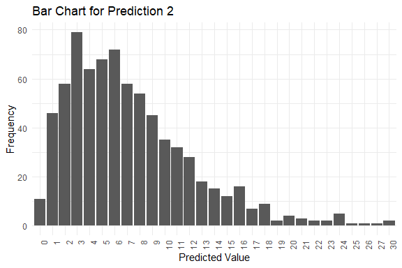
#>
#> $plots[[3]]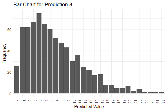
#>
#> $plots[[4]]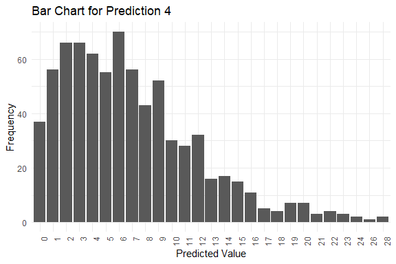
#>
#> $plots[[5]]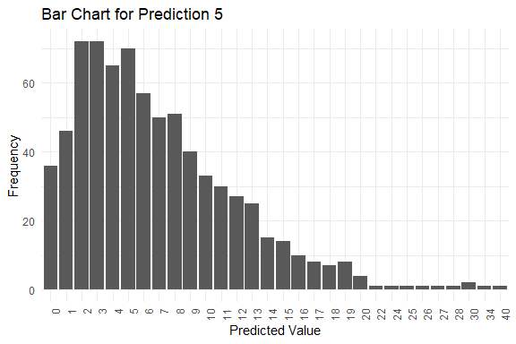
These binaries (installable software) and packages are in development.
They may not be fully stable and should be used with caution. We make no claims about them.
Health stats visible at Monitor.