The hardware and bandwidth for this mirror is donated by dogado GmbH, the Webhosting and Full Service-Cloud Provider. Check out our Wordpress Tutorial.
If you wish to report a bug, or if you are interested in having us mirror your free-software or open-source project, please feel free to contact us at mirror[@]dogado.de.
TOmicsVis: TranscriptOmics Visualization.
Website: https://benben-miao.github.io/TOmicsVis/
New!!! TOmicsVis Shinyapp:
# Start shiny application.
TOmicsVis::tomicsvis()1.2.1 Install required packages from Bioconductor:
# Install required packages from Bioconductor
install.packages("BiocManager")
BiocManager::install(c("ComplexHeatmap", "EnhancedVolcano", "clusterProfiler", "enrichplot", "impute", "preprocessCore", "Mfuzz"))
1.2.2 Github: https://github.com/benben-miao/TOmicsVis/
Install from Github:
install.packages("devtools")
devtools::install_github("benben-miao/TOmicsVis")

# Resolve network by GitClone
devtools::install_git("https://gitclone.com/github.com/benben-miao/TOmicsVis.git")
1.2.3 CRAN: https://cran.r-project.org/package=TOmicsVis
Install from CRAN:
# Install from CRAN
install.packages("TOmicsVis")Videos Courses: https://space.bilibili.com/34105515/channel/series
Article Introduction: 全解TOmicsVis完美应用于转录组可视化R包
Article Courses: TOmicsVis 转录组学R代码分析及可视化视频
OmicsSuite: Omics Suite Github: https://github.com/omicssuite/
Authors:
# 1. Library TOmicsVis package
library(TOmicsVis)
#> 载入需要的程辑包:Biobase
#> 载入需要的程辑包:BiocGenerics
#>
#> 载入程辑包:'BiocGenerics'
#> The following objects are masked from 'package:stats':
#>
#>     IQR, mad, sd, var, xtabs
#> The following objects are masked from 'package:base':
#>
#>     anyDuplicated, aperm, append, as.data.frame, basename, cbind,
#>     colnames, dirname, do.call, duplicated, eval, evalq, Filter, Find,
#>     get, grep, grepl, intersect, is.unsorted, lapply, Map, mapply,
#>     match, mget, order, paste, pmax, pmax.int, pmin, pmin.int,
#>     Position, rank, rbind, Reduce, rownames, sapply, setdiff, sort,
#>     table, tapply, union, unique, unsplit, which.max, which.min
#> Welcome to Bioconductor
#>
#>     Vignettes contain introductory material; view with
#>     'browseVignettes()'. To cite Bioconductor, see
#>     'citation("Biobase")', and for packages 'citation("pkgname")'.
#> 载入需要的程辑包:e1071
#>
#> Registered S3 method overwritten by 'GGally':
#>   method from
#>   +.gg   ggplot2
#>
#> 载入程辑包:'DynDoc'
#> The following object is masked from 'package:BiocGenerics':
#>
#>     path

# 2. Extra package
# install.packages("ggplot2")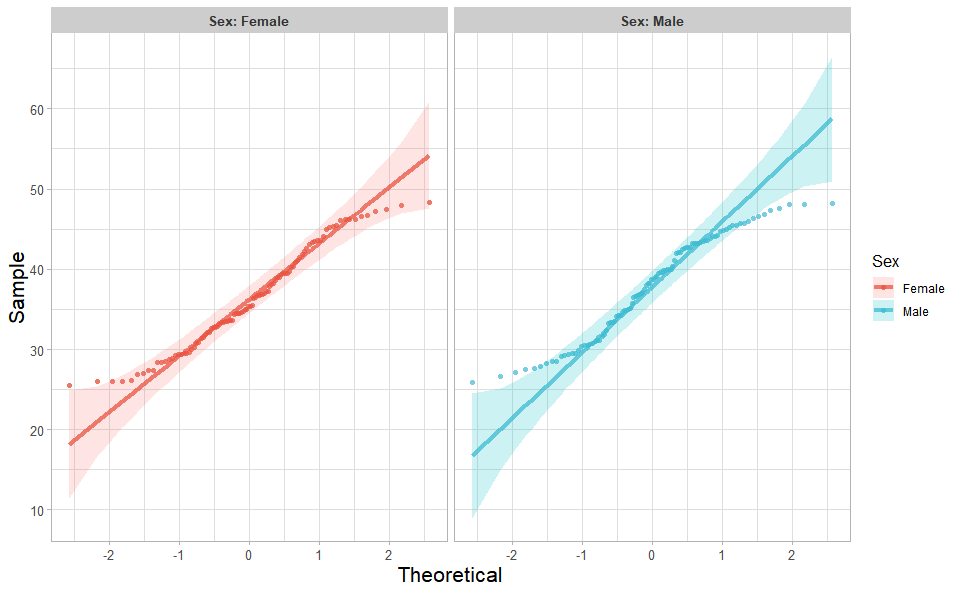
library(ggplot2)Input Data: Dataframe: Weight and Sex traits dataframe (1st-col: Weight, 2nd-col: Sex).
Output Plot: Quantile plot for visualizing data distribution.
# 1. Load example datasets
data(weight_sex)
head(weight_sex)
#>   Weight    Sex
#> 1  36.74 Female
#> 2  38.54 Female
#> 3  44.91 Female
#> 4  43.53 Female
#> 5  39.03 Female
#> 6  26.01 Female

# 2. Run quantile_plot plot function
quantile_plot(
  data = weight_sex,
  my_shape = "fill_circle",
  point_size = 1.5,
  conf_int = TRUE,
  conf_level = 0.95,
  split_panel = "Split_Panel",
  legend_pos = "right",
  legend_dir = "vertical",
  sci_fill_color = "Sci_NPG",
  sci_color_alpha = 0.75,
  ggTheme = "theme_light"
)
Get help using command ?TOmicsVis::quantile_plot or
reference page https://benben-miao.github.io/TOmicsVis/reference/quantile_plot.html.
# Get help with command in R console.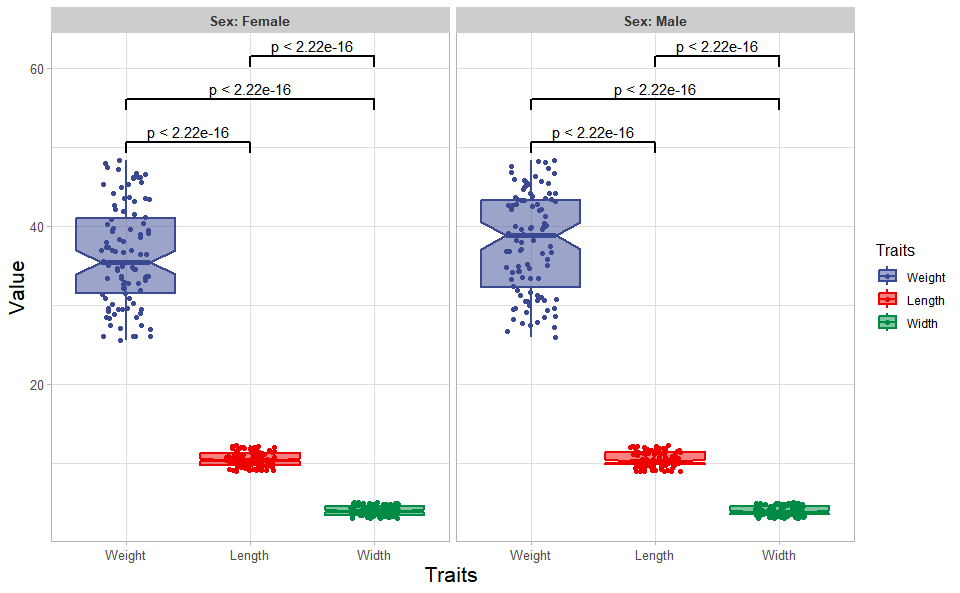
# ?TOmicsVis::quantile_plotInput Data: Dataframe: Length, Width, Weight, and Sex traits dataframe (1st-col: Value, 2nd-col: Traits, 3rd-col: Sex).
Output Plot: Plot: Box plot support two levels and multiple groups with P value.
# 1. Load example datasets
data(traits_sex)
head(traits_sex)
#>   Value Traits    Sex
#> 1 36.74 Weight Female
#> 2 38.54 Weight Female
#> 3 44.91 Weight Female
#> 4 43.53 Weight Female
#> 5 39.03 Weight Female
#> 6 26.01 Weight Female

# 2. Run box_plot plot function
box_plot(
  data = traits_sex,
  test_method = "t.test",
  test_label = "p.format",
  notch = TRUE,
  group_level = "Three_Column",
  add_element = "jitter",
  my_shape = "fill_circle",
  sci_fill_color = "Sci_AAAS",
  sci_fill_alpha = 0.5,
  sci_color_alpha = 1,
  legend_pos = "right",
  legend_dir = "vertical",
  ggTheme = "theme_light"
)
Get help using command ?TOmicsVis::box_plot or reference
page https://benben-miao.github.io/TOmicsVis/reference/box_plot.html.
# Get help with command in R console.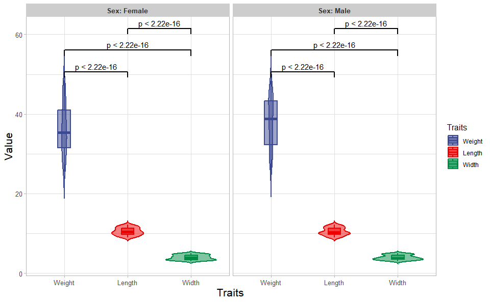
# ?TOmicsVis::box_plotInput Data: Dataframe: Length, Width, Weight, and Sex traits dataframe (1st-col: Value, 2nd-col: Traits, 3rd-col: Sex).
Output Plot: Plot: Violin plot support two levels and multiple groups with P value.
# 1. Load example datasets
data(traits_sex)

# 2. Run violin_plot plot function
violin_plot(
  data = traits_sex,
  test_method = "t.test",
  test_label = "p.format",
  group_level = "Three_Column",
  violin_orientation = "vertical",
  add_element = "boxplot",
  element_alpha = 0.5,
  my_shape = "plus_times",
  sci_fill_color = "Sci_AAAS",
  sci_fill_alpha = 0.5,
  sci_color_alpha = 1,
  legend_pos = "right",
  legend_dir = "vertical",
  ggTheme = "theme_light"
)
Get help using command ?TOmicsVis::violin_plot or
reference page https://benben-miao.github.io/TOmicsVis/reference/violin_plot.html.
# Get help with command in R console.
# ?TOmicsVis::violin_plotInput Data: Dataframe: survival record data (1st-col: Time, 2nd-col: Status, 3rd-col: Group).
Output Plot: Survival plot for analyzing and visualizing survival data.
# 1. Load example datasets
data(survival_data)
head(survival_data)
#>   Time Status Group
#> 1   48      0    CT
#> 2   48      0    CT
#> 3   48      0    CT
#> 4   48      0    CT
#> 5   48      0    CT
#> 6   48      0    CT

# 2. Run survival_plot plot function
survival_plot(
  data = survival_data,
  curve_function = "pct",
  conf_inter = TRUE,
  interval_style = "ribbon",
  risk_table = TRUE,
  num_censor = TRUE,
  sci_palette = "aaas",
  ggTheme = "theme_light",
  x_start = 0,
  y_start = 0,
  y_end = 100,
  x_break = 10,
  y_break = 10
)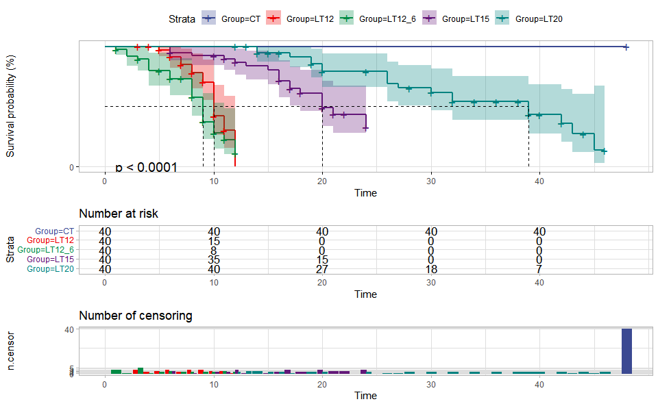
Get help using command ?TOmicsVis::survival_plot or
reference page https://benben-miao.github.io/TOmicsVis/reference/survival_plot.html.
# Get help with command in R console.
# ?TOmicsVis::survival_plotInput Data: Dataframe: All genes in all samples expression dataframe of RNA-Seq (1st-col: Genes, 2nd-col~: Samples).
Output Plot: Plot: heatmap plot filled with Pearson correlation values and P values.
# 1. Load example dataset
data(gene_expression)
head(gene_expression)
#>              Genes   CT_1   CT_2   CT_3 LT20_1 LT20_2 LT20_3 LT15_1 LT15_2
#> 1     transcript_0 655.78 631.08 669.89 654.21 402.56 447.09 510.08 442.22
#> 2     transcript_1  92.72 112.26 150.30  88.35  76.35  94.55 120.24  80.89
#> 3    transcript_10  21.74  31.11  22.58  15.09  13.67  13.24  12.48   7.53
#> 4   transcript_100   0.00   0.00   0.00   0.00   0.00   0.00   0.00   0.00
#> 5  transcript_1000   0.00  14.15  36.01   0.00   0.00 193.59 208.45   0.00
#> 6 transcript_10000  89.18 158.04  86.28  82.97 117.78 102.24 129.61 112.73
#>   LT15_3 LT12_1 LT12_2 LT12_3 LT12_6_1 LT12_6_2 LT12_6_3
#> 1 399.82 483.30 437.89 444.06   405.43   416.63   464.75
#> 2  73.94  96.25  82.62  85.48    65.12    61.94    73.44
#> 3  13.35  11.16  11.36   6.96     7.82     4.01    10.02
#> 4   0.00   0.00   0.00   0.00     0.00     0.00     0.00
#> 5 232.40 148.58   0.00 181.61     0.02    12.18     0.00
#> 6  85.70  80.89 124.11 115.25   113.87   107.69   119.83

# 2. Run corr_heatmap plot function
corr_heatmap(
  data = gene_expression,
  corr_method = "pearson",
  cell_shape = "square",
  fill_type = "full",
  lable_size = 3,
  axis_angle = 45,
  axis_size = 12,
  lable_digits = 3,
  color_low = "blue",
  color_mid = "white",
  color_high = "red",
  outline_color = "white",
  ggTheme = "theme_light"
)
#> Scale for fill is already present.
#> Adding another scale for fill, which will replace the existing scale.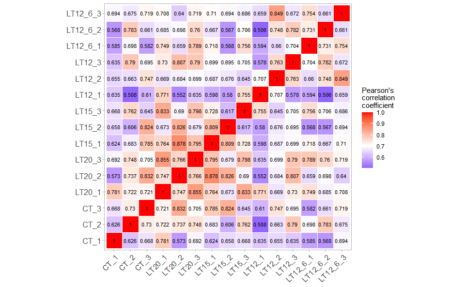
Get help using command ?TOmicsVis::corr_heatmap or
reference page https://benben-miao.github.io/TOmicsVis/reference/corr_heatmap.html.
# Get help with command in R console.
# ?TOmicsVis::corr_heatmapInput Data1: Dataframe: All genes in all samples expression dataframe of RNA-Seq (1st-col: Genes, 2nd-col~: Samples).
Input Data2: Dataframe: Samples and groups for gene expression (1st-col: Samples, 2nd-col: Groups).
Output Table: PCA dimensional reduction analysis for RNA-Seq.
# 1. Load example datasets
data(gene_expression)

data(samples_groups)
head(samples_groups)
#>   Samples Groups
#> 1    CT_1     CT
#> 2    CT_2     CT
#> 3    CT_3     CT
#> 4  LT20_1   LT20
#> 5  LT20_2   LT20
#> 6  LT20_3   LT20

# 2. Run pca_analysis plot function
res <- pca_analysis(gene_expression, samples_groups)
head(res)
#>               PC1         PC2         PC3        PC4         PC5       PC6
#> CT_1   -27010.536 -18328.2803   5955.2569 46547.7319  11394.1043 -7197.285
#> CT_2    16248.651  29132.9251   -824.1857 20747.9618 -18798.8755 21096.088
#> CT_3    22421.017 -26832.3964   6789.4490  5864.1171 -15375.3418 17424.861
#> LT20_1 -18587.073   -472.9036 -21638.7836  7765.9575    114.1225 -3943.968
#> LT20_2  33275.933  -9874.9959 -14991.3942 -7443.9250  -4600.8302 -8072.298
#> LT20_3  -1596.255  11683.5426 -10892.8493   381.0795  11080.3560 -8994.187
#>                PC7        PC8        PC9        PC10        PC11       PC12
#> CT_1     2150.6739   4850.320   4051.745   7666.9445  -3141.9327  -2487.939
#> CT_2   -12329.1138  -3353.734   4805.659   1503.8533  11184.0296  -4865.436
#> CT_3    12744.2255 -10037.516 -11468.842    202.4016 -11001.6260  -3847.291
#> LT20_1   8864.7482 -14171.127  -1968.082  -3562.1899   7446.2105  14831.486
#> LT20_2   -941.3943  -5072.401   5345.106   6494.1383  -3954.2153   9351.346
#> LT20_3   7263.9321  -7774.725  -1853.546 -21427.2641    -46.1503 -12507.011
#>              PC13       PC14          PC15
#> CT_1    -2704.613  2396.7383  2.528517e-11
#> CT_2    -2633.057 -1375.3352  6.825657e-11
#> CT_3     5193.978   188.5601  2.255671e-11
#> LT20_1   3937.457 -7871.8062  4.864246e-11
#> LT20_2 -12904.673  6071.6618 -2.020696e-10
#> LT20_3  -5369.380  2606.1762  1.903509e-11
Get help using command ?TOmicsVis::pca_analysis or
reference page https://benben-miao.github.io/TOmicsVis/reference/pca_analysis.html.
# Get help with command in R console.
# ?TOmicsVis::pca_analysisInput Data1: Dataframe: All genes in all samples expression dataframe of RNA-Seq (1st-col: Genes, 2nd-col~: Samples).
Input Data2: Dataframe: Samples and groups for gene expression (1st-col: Samples, 2nd-col: Groups).
Output Plot: Plot: PCA dimensional reduction visualization for RNA-Seq.
# 1. Load example datasets
data(gene_expression)

data(samples_groups)
head(samples_groups)
#>   Samples Groups
#> 1    CT_1     CT
#> 2    CT_2     CT
#> 3    CT_3     CT
#> 4  LT20_1   LT20
#> 5  LT20_2   LT20
#> 6  LT20_3   LT20

# 2. Run pca_plot plot function
pca_plot(
  sample_gene = gene_expression,
  group_sample = samples_groups,
  xPC = 1,
  yPC = 2,
  point_size = 5,
  text_size = 5,
  fill_alpha = 0.10,
  border_alpha = 0.00,
  legend_pos = "right",
  legend_dir = "vertical",
  ggTheme = "theme_light"
)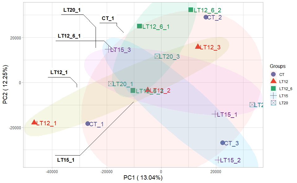
Get help using command ?TOmicsVis::pca_plot or reference
page https://benben-miao.github.io/TOmicsVis/reference/pca_plot.html.
# Get help with command in R console.
# ?TOmicsVis::pca_plotInput Data1: Dataframe: All genes in all samples expression dataframe of RNA-Seq (1st-col: Genes, 2nd-col~: Samples).
Input Data2: Dataframe: Samples and groups for gene expression (1st-col: Samples, 2nd-col: Groups).
Output Table: TSNE analysis for analyzing and visualizing TSNE algorithm.
# 1. Load example datasets
data(gene_expression)
data(samples_groups)

# 2. Run tsne_analysis plot function
res <- tsne_analysis(gene_expression, samples_groups)
head(res)
#>       TSNE1     TSNE2
#> 1 -67.41252 -16.61397
#> 2  43.08349 -34.02654
#> 3 123.32273  54.14358
#> 4 -42.52065 -31.30027
#> 5  94.98790  48.97986
#> 6 -23.90637 -22.26434
Get help using command ?TOmicsVis::tsne_analysis or
reference page https://benben-miao.github.io/TOmicsVis/reference/tsne_analysis.html.
# Get help with command in R console.
# ?TOmicsVis::tsne_analysisInput Data1: Dataframe: All genes in all samples expression dataframe of RNA-Seq (1st-col: Genes, 2nd-col~: Samples).
Input Data2: Dataframe: Samples and groups for gene expression (1st-col: Samples, 2nd-col: Groups).
Output Plot: TSNE plot for analyzing and visualizing TSNE algorithm.
# 1. Load example datasets
data(gene_expression)
data(samples_groups)

# 2. Run tsne_plot plot function
tsne_plot(
  sample_gene = gene_expression,
  group_sample = samples_groups,
  seed = 1,
  multi_shape = FALSE,
  point_size = 5,
  point_alpha = 0.8,
  text_size = 5,
  text_alpha = 0.80,
  fill_alpha = 0.10,
  border_alpha = 0.00,
  sci_fill_color = "Sci_AAAS",
  legend_pos = "right",
  legend_dir = "vertical",
  ggTheme = "theme_light"
)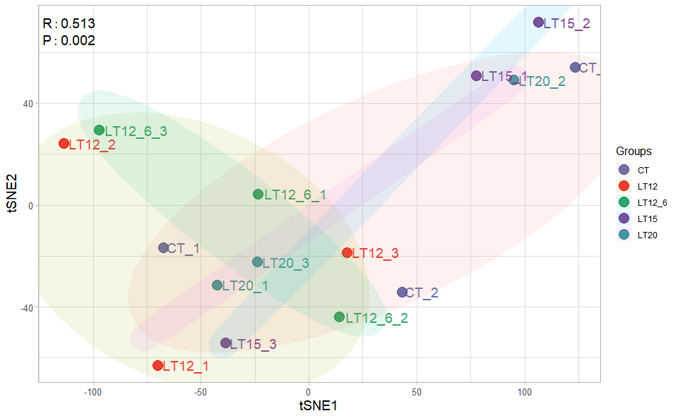
Get help using command ?TOmicsVis::tsne_plot or
reference page https://benben-miao.github.io/TOmicsVis/reference/tsne_plot.html.
# Get help with command in R console.
# ?TOmicsVis::tsne_plotInput Data1: Dataframe: All genes in all samples expression dataframe of RNA-Seq (1st-col: Genes, 2nd-col~: Samples).
Input Data2: Dataframe: Samples and groups for gene expression (1st-col: Samples, 2nd-col: Groups).
Output Table: UMAP analysis for analyzing RNA-Seq data.
# 1. Load example datasets
data(gene_expression)
data(samples_groups)

# 2. Run tsne_plot plot function
res <- umap_analysis(gene_expression, samples_groups)
head(res)
#>             UMAP1       UMAP2
#> CT_1   -0.6752746  0.49425898
#> CT_2    1.0232441  0.03062202
#> CT_3   -0.4722297 -1.32183550
#> LT20_1 -0.2414214  0.13870703
#> LT20_2  0.1991701 -1.23434000
#> LT20_3  0.6431577  1.11879669
Get help using command ?TOmicsVis::umap_analysis or
reference page https://benben-miao.github.io/TOmicsVis/reference/umap_analysis.html.
# Get help with command in R console.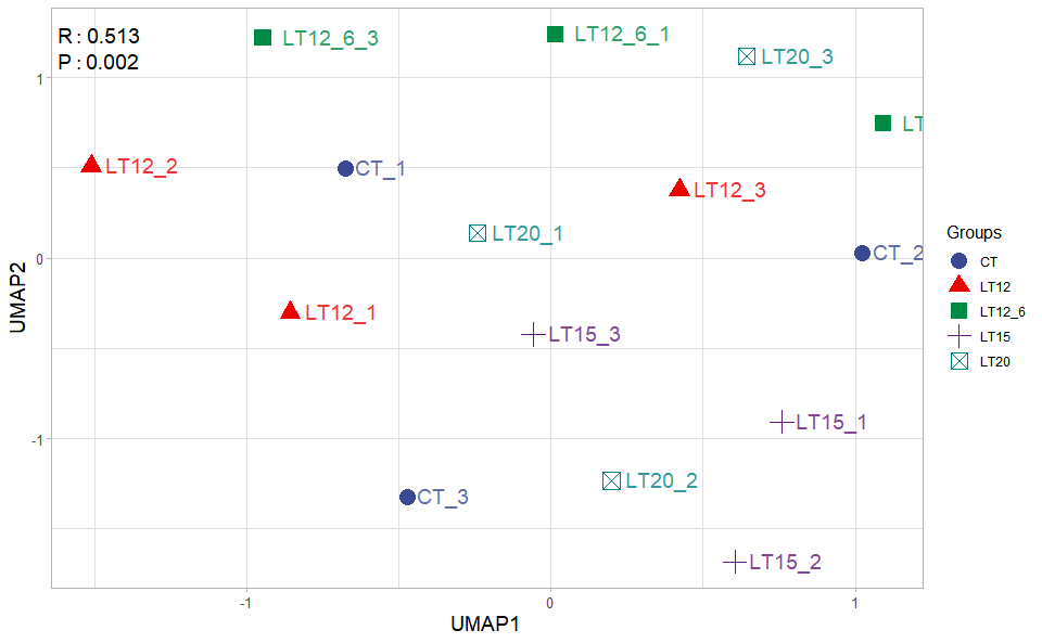
# ?TOmicsVis::umap_analysisInput Data1: Dataframe: All genes in all samples expression dataframe of RNA-Seq (1st-col: Genes, 2nd-col~: Samples).
Input Data2: Dataframe: Samples and groups for gene expression (1st-col: Samples, 2nd-col: Groups).
Output Plot: UMAP plot for analyzing and visualizing UMAP algorithm.
# 1. Load example datasets
data(gene_expression)
data(samples_groups)

# 2. Run tsne_plot plot function
umap_plot(
  sample_gene = gene_expression,
  group_sample = samples_groups,
  seed = 1,
  multi_shape = TRUE,
  point_size = 5,
  point_alpha = 1,
  text_size = 5,
  text_alpha = 0.80,
  fill_alpha = 0.00,
  border_alpha = 0.00,
  sci_fill_color = "Sci_AAAS",
  legend_pos = "right",
  legend_dir = "vertical",
  ggTheme = "theme_light"
)
Get help using command ?TOmicsVis::umap_plot or
reference page https://benben-miao.github.io/TOmicsVis/reference/umap_plot.html.
# Get help with command in R console.
# ?TOmicsVis::umap_plotInput Data: Dataframe: All genes in all samples expression dataframe of RNA-Seq (1st-col: Genes, 2nd-col~: Samples).
Output Plot: Plot: dendrogram for multiple samples clustering.
# 1. Load example datasets
data(gene_expression)

# 2. Run plot function
dendro_plot(
  data = gene_expression,
  dist_method = "euclidean",
  hc_method = "ward.D2",
  tree_type = "rectangle",
  k_num = 5,
  palette = "npg",
  color_labels_by_k = TRUE,
  horiz = FALSE,
  label_size = 1,
  line_width = 1,
  rect = TRUE,
  rect_fill = TRUE,
  xlab = "Samples",
  ylab = "Height",
  ggTheme = "theme_light"
)
#> Registered S3 method overwritten by 'dendextend':
#>   method     from
#>   rev.hclust vegan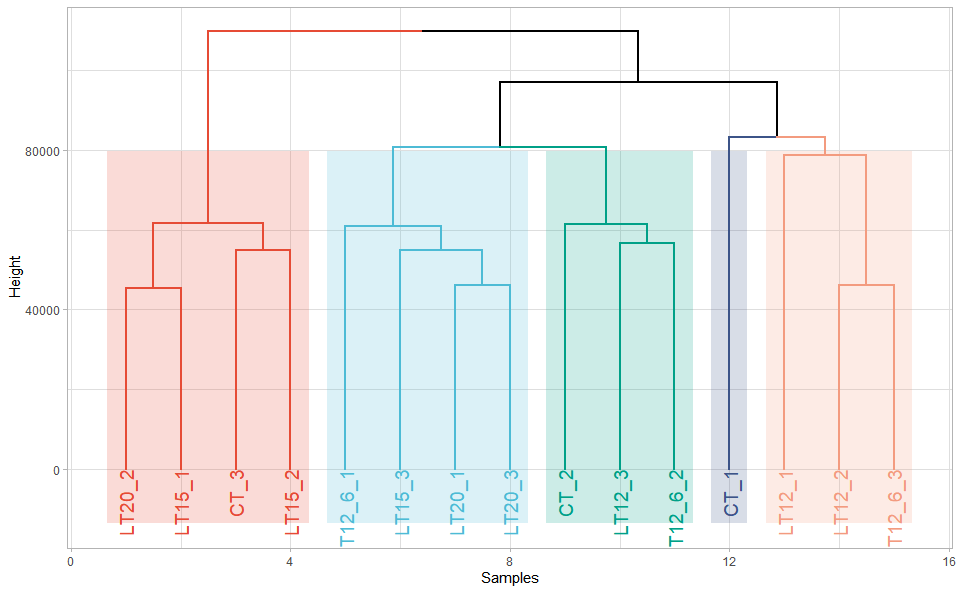
Get help using command ?TOmicsVis::dendro_plot or
reference page https://benben-miao.github.io/TOmicsVis/reference/dendro_plot.html.
# Get help with command in R console.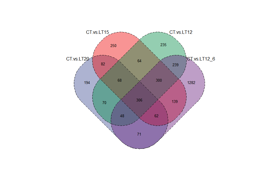
# ?TOmicsVis::dendro_plotInput Data2: Dataframe: Paired comparisons differentially expressed genes (degs) among groups (1st-col~: degs of paired comparisons).
Output Plot: Venn plot for stat common and unique gene among multiple sets.
# 1. Load example datasets
data(degs_lists)
head(degs_lists)
#>        CT.vs.LT20      CT.vs.LT15       CT.vs.LT12     CT.vs.LT12_6
#> 1 transcript_9024 transcript_4738  transcript_9956 transcript_10354
#> 2  transcript_604 transcript_6050  transcript_7601  transcript_2959
#> 3 transcript_3912 transcript_1039  transcript_5960  transcript_5919
#> 4 transcript_8676 transcript_1344  transcript_3240  transcript_2395
#> 5 transcript_8832 transcript_3069 transcript_10224  transcript_9881
#> 6   transcript_74 transcript_9809  transcript_3151  transcript_8836

# 2. Run venn_plot plot function
venn_plot(
  data = degs_lists,
    title_size = 1,
    label_show = TRUE,
    label_size = 0.8,
    border_show = TRUE,
    line_type = "longdash",
    ellipse_shape = "circle",
    sci_fill_color = "Sci_AAAS",
    sci_fill_alpha = 0.65
)
Get help using command ?TOmicsVis::venn_plot or
reference page https://benben-miao.github.io/TOmicsVis/reference/venn_plot.html.
# Get help with command in R console.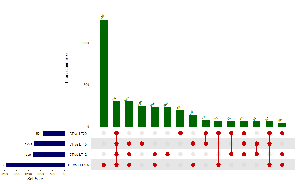
# ?TOmicsVis::venn_plotInput Data2: Dataframe: Paired comparisons differentially expressed genes (degs) among groups (1st-col~: degs of paired comparisons).
Output Plot: UpSet plot for stat common and unique gene among multiple sets.
# 1. Load example datasets
data(degs_lists)
head(degs_lists)
#>        CT.vs.LT20      CT.vs.LT15       CT.vs.LT12     CT.vs.LT12_6
#> 1 transcript_9024 transcript_4738  transcript_9956 transcript_10354
#> 2  transcript_604 transcript_6050  transcript_7601  transcript_2959
#> 3 transcript_3912 transcript_1039  transcript_5960  transcript_5919
#> 4 transcript_8676 transcript_1344  transcript_3240  transcript_2395
#> 5 transcript_8832 transcript_3069 transcript_10224  transcript_9881
#> 6   transcript_74 transcript_9809  transcript_3151  transcript_8836

# 2. Run upsetr_plot plot function
upsetr_plot(
  data = degs_lists,
  sets_num = 4,
  keep_order = FALSE,
  order_by = "freq",
  decrease = TRUE,
  mainbar_color = "#006600",
  number_angle = 45,
  matrix_color = "#cc0000",
  point_size = 4.5,
  point_alpha = 0.5,
  line_size = 0.8,
  shade_color = "#cdcdcd",
  shade_alpha = 0.5,
  setsbar_color = "#000066",
  setsnum_size = 6,
  text_scale = 1.2
)
Get help using command ?TOmicsVis::upsetr_plot or
reference page https://benben-miao.github.io/TOmicsVis/reference/upsetr_plot.html.
# Get help with command in R console.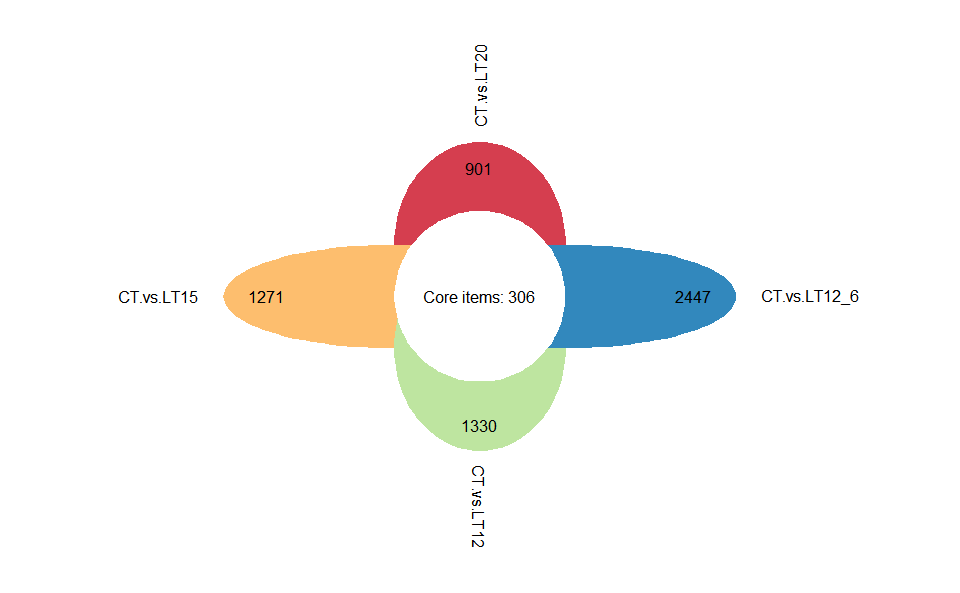
# ?TOmicsVis::upsetr_plotInput Data2: Dataframe: Paired comparisons differentially expressed genes (degs) among groups (1st-col~: degs of paired comparisons).
Output Plot: Flower plot for stat common and unique gene among multiple sets.
# 1. Load example datasets
data(degs_lists)

# 2. Run plot function
flower_plot(
  flower_dat = degs_lists,
  angle = 90,
  a = 1,
  b = 2,
  r = 1,
  ellipse_col_pal = "Spectral",
  circle_col = "white",
  label_text_cex = 1
)
Get help using command ?TOmicsVis::flower_plot or
reference page https://benben-miao.github.io/TOmicsVis/reference/flower_plot.html.
# Get help with command in R console.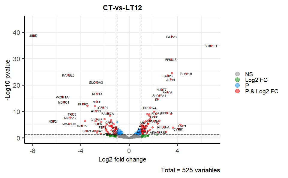
# ?TOmicsVis::flower_plotInput Data2: Dataframe: All DEGs of paired comparison CT-vs-LT12 stats dataframe (1st-col: Genes, 2nd-col: log2FoldChange, 3rd-col: Pvalue, 4th-col: FDR).
Output Plot: Volcano plot for visualizing differentailly expressed genes.
# 1. Load example datasets
data(degs_stats)
head(degs_stats)
#>    Gene log2FoldChange      Pvalue         FDR
#> 1  A1I3    -1.13855748 0.000111040 0.000862478
#> 2   A1M     0.59076131 0.070988041 0.192551708
#> 3   A2M     0.09297827 0.819706797 0.913893947
#> 4 A2ML1    -0.26940689 0.745374782 0.874295125
#> 5  ABAT     1.24811621 0.000001440 0.000016800
#> 6 ABCC3    -0.72947545 0.005171574 0.024228298

# 2. Run volcano_plot plot function
volcano_plot(
  data = degs_stats,
  title = "CT-vs-LT12",
  log2fc_cutoff = 1,
  pq_value = "pvalue",
  pq_cutoff = 0.05,
  cutoff_line = "longdash",
  point_shape = "large_circle",
  point_size = 2,
  point_alpha = 0.5,
  color_normal = "#888888",
  color_log2fc = "#008000",
  color_pvalue = "#0088ee",
  color_Log2fc_p = "#ff0000",
  label_size = 3,
  boxed_labels = FALSE,
  draw_connectors = FALSE,
  legend_pos = "right"
)
Get help using command ?TOmicsVis::volcano_plot or
reference page https://benben-miao.github.io/TOmicsVis/reference/volcano_plot.html.
# Get help with command in R console.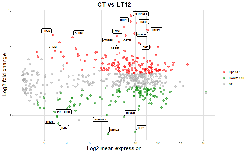
# ?TOmicsVis::volcano_plotInput Data2: Dataframe: All DEGs of paired comparison CT-vs-LT12 stats2 dataframe (1st-col: Gene, 2nd-col: baseMean, 3rd-col: Log2FoldChange, 4th-col: FDR).
Output Plot: MversusA plot for visualizing differentially expressed genes.
# 1. Load example datasets
data(degs_stats2)
head(degs_stats2)
#>    name     baseMean log2FoldChange         padj
#> 1  A1I3    0.1184475      0.0000000           NA
#> 2   A1M 1654.4618140      0.6789538 5.280802e-02
#> 3   A2M  681.0463277      1.5263838 3.920000e-07
#> 4 A2ML1  389.7226640      3.8933573 1.180000e-14
#> 5  ABAT  364.7810090     -2.3554014 1.559230e-04
#> 6 ABCC3    1.1346239      1.2932740 4.491812e-01

# 2. Run volcano_plot plot function
ma_plot(
  data = degs_stats2,
  foldchange = 2,
  fdr_value = 0.05,
  point_size = 3.0,
  color_up = "#FF0000",
  color_down = "#008800",
  color_alpha = 0.5,
  top_method = "fc",
  top_num = 20,
  label_size = 8,
  label_box = TRUE,
  title = "CT-vs-LT12",
  xlab = "Log2 mean expression",
  ylab = "Log2 fold change",
  ggTheme = "theme_light"
)
Get help using command ?TOmicsVis::ma_plot or reference
page https://benben-miao.github.io/TOmicsVis/reference/ma_plot.html.
# Get help with command in R console.
# ?TOmicsVis::ma_plotInput Data1: Dataframe: Shared DEGs of all paired comparisons in all samples expression dataframe of RNA-Seq. (1st-col: Genes, 2nd-col~: Samples).
Input Data2: Dataframe: Samples and groups for gene expression (1st-col: Samples, 2nd-col: Groups).
Output Plot: Heatmap group for visualizing grouped gene expression data.
# 1. Load example datasets
data(gene_expression2)
data(samples_groups)

# 2. Run heatmap_group plot function
heatmap_group(
  sample_gene = gene_expression2[1:30,],
  group_sample = samples_groups,
  scale_data = "row",
  clust_method = "complete",
  border_show = TRUE,
  border_color = "#ffffff",
  value_show = TRUE,
  value_decimal = 2,
  value_size = 5,
  axis_size = 8,
  cell_height = 10,
  low_color = "#00880055",
  mid_color = "#ffffff",
  high_color = "#ff000055",
  na_color = "#ff8800",
  x_angle = 45
)
Get help using command ?TOmicsVis::heatmap_group or
reference page https://benben-miao.github.io/TOmicsVis/reference/heatmap_group.html.
# Get help with command in R console.
# ?TOmicsVis::heatmap_groupInput Data2: Dataframe: Shared DEGs of all paired comparisons in all samples expression dataframe of RNA-Seq. (1st-col: Genes, 2nd-col~: Samples).
Output Plot: Circos heatmap plot for visualizing gene expressing in multiple samples.
# 1. Load example datasets
data(gene_expression2)
head(gene_expression2)
#>   Genes  CT_1    CT_2  CT_3 LT20_1 LT20_2 LT20_3 LT15_1 LT15_2 LT15_3 LT12_1
#> 1 ACAA2 24.50   39.83 55.38 114.11 159.32  96.88 169.56 464.84 182.66 116.08
#> 2  ACAN 14.97   18.71 10.30  71.23 142.67 213.54 253.15 320.80 104.15 174.02
#> 3  ADH1  1.54    1.56  2.04  14.95  13.60  15.87  12.80  17.74   6.06  10.97
#> 4  AHSG  0.00 1911.99  0.00   0.00   0.00   0.00   0.00   0.00   0.00   0.00
#> 5 ALDH2  2.07    2.86  2.54   0.85   0.49   0.47   0.42   0.13   0.26   0.00
#> 6 AP1S3  6.62   14.59  9.30  24.90  33.94  23.19  24.00  36.08  27.40  24.06
#>   LT12_2 LT12_3 LT12_6_1 LT12_6_2 LT12_6_3
#> 1 497.29 464.48   471.43   693.62   229.77
#> 2 305.81 469.48  1291.90   991.90   966.77
#> 3  10.71  30.95     9.84    10.91     7.28
#> 4   0.00   0.00     0.00     0.00     0.00
#> 5   0.28   0.11     0.37     0.15     0.11
#> 6  38.74  34.54    62.72    41.36    28.75

# 2. Run circos_heatmap plot function
circos_heatmap(
  data = gene_expression2[1:50,],
  low_color = "#0000ff",
  mid_color = "#ffffff",
  high_color = "#ff0000",
  gap_size = 25,
  cluster_run = TRUE,
  cluster_method = "complete",
  distance_method = "euclidean",
  dend_show = "inside",
  dend_height = 0.2,
  track_height = 0.3,
  rowname_show = "outside",
  rowname_size = 0.8
)
#> Note: 15 points are out of plotting region in sector 'group', track
#> '3'.
#> Note: 15 points are out of plotting region in sector 'group', track
#> '3'.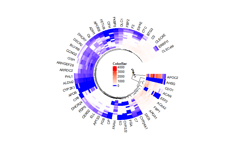
Get help using command ?TOmicsVis::circos_heatmap or
reference page https://benben-miao.github.io/TOmicsVis/reference/circos_heatmap.html.
# Get help with command in R console.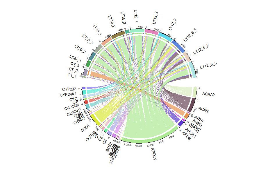
# ?TOmicsVis::circos_heatmapInput Data2: Dataframe: Shared DEGs of all paired comparisons in all samples expression dataframe of RNA-Seq. (1st-col: Genes, 2nd-col~: Samples).
Output Plot: Chord plot for visualizing the relationships of pathways and genes.
# 1. Load chord_data example datasets
data(gene_expression2)
head(gene_expression2)
#>   Genes  CT_1    CT_2  CT_3 LT20_1 LT20_2 LT20_3 LT15_1 LT15_2 LT15_3 LT12_1
#> 1 ACAA2 24.50   39.83 55.38 114.11 159.32  96.88 169.56 464.84 182.66 116.08
#> 2  ACAN 14.97   18.71 10.30  71.23 142.67 213.54 253.15 320.80 104.15 174.02
#> 3  ADH1  1.54    1.56  2.04  14.95  13.60  15.87  12.80  17.74   6.06  10.97
#> 4  AHSG  0.00 1911.99  0.00   0.00   0.00   0.00   0.00   0.00   0.00   0.00
#> 5 ALDH2  2.07    2.86  2.54   0.85   0.49   0.47   0.42   0.13   0.26   0.00
#> 6 AP1S3  6.62   14.59  9.30  24.90  33.94  23.19  24.00  36.08  27.40  24.06
#>   LT12_2 LT12_3 LT12_6_1 LT12_6_2 LT12_6_3
#> 1 497.29 464.48   471.43   693.62   229.77
#> 2 305.81 469.48  1291.90   991.90   966.77
#> 3  10.71  30.95     9.84    10.91     7.28
#> 4   0.00   0.00     0.00     0.00     0.00
#> 5   0.28   0.11     0.37     0.15     0.11
#> 6  38.74  34.54    62.72    41.36    28.75

# 2. Run chord_plot plot function
chord_plot(
  data = gene_expression2[1:30,],
  multi_colors = "VividColors",
  color_seed = 10,
  color_alpha = 0.3,
  link_visible = TRUE,
  link_dir = -1,
  link_type = "diffHeight",
  sector_scale = "Origin",
  width_circle = 3,
  dist_name = 3,
  label_dir = "Vertical",
  dist_label = 0.3,
  label_scale = 0.8
)
#>      rn   cn value1 value2 o1 o2      x1     x2       col
#> 1 ACAA2 CT_1  24.50  24.50 15 30 3779.75 394.66 #DAECC0B2
#> 2  ACAN CT_1  14.97  14.97 15 29 5349.40 370.16 #694858B2
#> 3  ADH1 CT_1   1.54   1.54 15 28  166.82 355.19 #C047A3B2
#> 4  AHSG CT_1   0.00   0.00 15 27 1911.99 353.65 #E7934EB2
#> 5 ALDH2 CT_1   2.07   2.07 15 26   11.11 353.65 #71EC4AB2
#> 6 AP1S3 CT_1   6.62   6.62 15 25  430.19 351.58 #D334EDB2
Get help using command ?TOmicsVis::chord_plot or
reference page https://benben-miao.github.io/TOmicsVis/reference/chord_plot.html.
# Get help with command in R console.
# ?TOmicsVis::chord_plotInput Data: Dataframe: All DEGs of paired comparison CT-vs-LT12 stats dataframe (1st-col: Genes, 2nd-col: log2FoldChange, 3rd-col: Pvalue, 4th-col: FDR).
Output Plot: Gene cluster trend plot for visualizing gene expression trend profile in multiple samples.
# 1. Load example datasets
data(degs_stats)

# 2. Run plot function
gene_rank_plot(
  data = degs_stats,
  log2fc = 1,
  palette = "Spectral",
  top_n = 10,
  genes_to_label = NULL,
  label_size = 5,
  base_size = 12,
  title = "Gene ranking dotplot",
  xlab = "Ranking of differentially expressed genes",
  ylab = "Log2FoldChange"
)![]()
Get help using command ?TOmicsVis::gene_rank_plot or
reference page https://benben-miao.github.io/TOmicsVis/reference/gene_rank_plot.html.
# Get help with command in R console.
# ?TOmicsVis::gene_rank_plotInput Data2: Dataframe: Shared DEGs of all paired comparisons in all groups expression dataframe of RNA-Seq. (1st-col: Genes, 2nd-col~n-1-col: Groups, n-col: Pathways).
Output Plot: Gene cluster trend plot for visualizing gene expression trend profile in multiple samples.
# 1. Load example datasets
data(gene_expression3)

# 2. Run plot function
gene_cluster_trend(
  data = gene_expression3[,-7],
  thres = 0.25,
  min_std = 0.2,
  palette = "PiYG",
  cluster_num = 4
)
#> 0 genes excluded.
#> 0 genes excluded.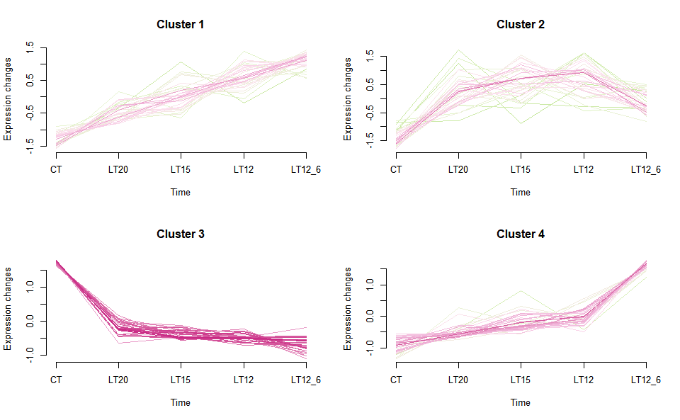
#> NULLGet help using command ?TOmicsVis::gene_cluster_trend or
reference page https://benben-miao.github.io/TOmicsVis/reference/gene_cluster_trend.html.
# Get help with command in R console.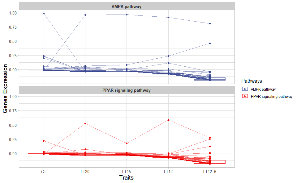
# ?TOmicsVis::gene_cluster_trendInput Data2: Dataframe: Shared DEGs of all paired comparisons in all groups expression dataframe of RNA-Seq. (1st-col: Genes, 2nd-col~n-1-col: Groups, n-col: Pathways).
Output Plot: Trend plot for visualizing gene expression trend profile in multiple traits.
# 1. Load example datasets
data(gene_expression3)
head(gene_expression3)
#>   Genes         CT        LT20     LT15      LT12      LT12_6
#> 1 ACAA2  39.903333 123.4366667 272.3533 359.28333  464.940000
#> 2  ACAN  14.660000 142.4800000 226.0333 316.43667 1083.523333
#> 3  ADH1   1.713333  14.8066667  12.2000  17.54333    9.343333
#> 4  AHSG 637.330000   0.0000000   0.0000   0.00000    0.000000
#> 5 ALDH2   2.490000   0.6033333   0.2700   0.13000    0.210000
#> 6 AP1S3  10.170000  27.3433333  29.1600  32.44667   44.276667
#>                 Pathways
#> 1 PPAR signaling pathway
#> 2 PPAR signaling pathway
#> 3 PPAR signaling pathway
#> 4 PPAR signaling pathway
#> 5 PPAR signaling pathway
#> 6 PPAR signaling pathway

# 2. Run trend_plot plot function
trend_plot(
  data = gene_expression3[1:100,],
  scale_method = "centerObs",
  miss_value = "exclude",
  line_alpha = 0.5,
  show_points = TRUE,
  show_boxplot = TRUE,
  num_column = 1,
  xlab = "Traits",
  ylab = "Genes Expression",
  sci_fill_color = "Sci_AAAS",
  sci_fill_alpha = 0.8,
  sci_color_alpha = 0.8,
  legend_pos = "right",
  legend_dir = "vertical",
  ggTheme = "theme_light"
)
Get help using command ?TOmicsVis::trend_plot or
reference page https://benben-miao.github.io/TOmicsVis/reference/trend_plot.html.
# Get help with command in R console.
# ?TOmicsVis::trend_plotInput Data1: Dataframe: All genes in all samples expression dataframe of RNA-Seq (1st-col: Genes, 2nd-col~: Samples).
Input Data2: Dataframe: Samples and groups for gene expression (1st-col: Samples, 2nd-col: Groups).
Output Plot: WGCNA analysis pipeline for RNA-Seq.
# 1. Load wgcna_pipeline example datasets
data(gene_expression)
head(gene_expression)
#>              Genes   CT_1   CT_2   CT_3 LT20_1 LT20_2 LT20_3 LT15_1 LT15_2
#> 1     transcript_0 655.78 631.08 669.89 654.21 402.56 447.09 510.08 442.22
#> 2     transcript_1  92.72 112.26 150.30  88.35  76.35  94.55 120.24  80.89
#> 3    transcript_10  21.74  31.11  22.58  15.09  13.67  13.24  12.48   7.53
#> 4   transcript_100   0.00   0.00   0.00   0.00   0.00   0.00   0.00   0.00
#> 5  transcript_1000   0.00  14.15  36.01   0.00   0.00 193.59 208.45   0.00
#> 6 transcript_10000  89.18 158.04  86.28  82.97 117.78 102.24 129.61 112.73
#>   LT15_3 LT12_1 LT12_2 LT12_3 LT12_6_1 LT12_6_2 LT12_6_3
#> 1 399.82 483.30 437.89 444.06   405.43   416.63   464.75
#> 2  73.94  96.25  82.62  85.48    65.12    61.94    73.44
#> 3  13.35  11.16  11.36   6.96     7.82     4.01    10.02
#> 4   0.00   0.00   0.00   0.00     0.00     0.00     0.00
#> 5 232.40 148.58   0.00 181.61     0.02    12.18     0.00
#> 6  85.70  80.89 124.11 115.25   113.87   107.69   119.83

data(samples_groups)
head(samples_groups)
#>   Samples Groups
#> 1    CT_1     CT
#> 2    CT_2     CT
#> 3    CT_3     CT
#> 4  LT20_1   LT20
#> 5  LT20_2   LT20
#> 6  LT20_3   LT20

# 2. Run wgcna_pipeline plot function
# wgcna_pipeline(gene_expression[1:3000,], samples_groups)
Get help using command ?TOmicsVis::wgcna_pipeline or
reference page https://benben-miao.github.io/TOmicsVis/reference/wgcna_pipeline.html.
# Get help with command in R console.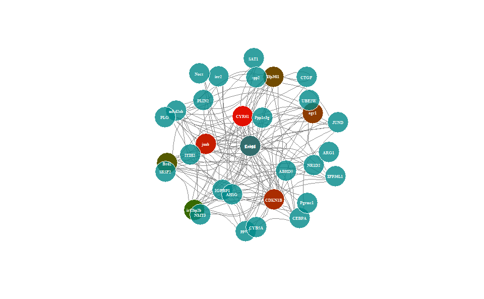
# ?TOmicsVis::wgcna_pipelineInput Data: Dataframe: Network data from WGCNA tan module top-200 dataframe (1st-col: Source, 2nd-col: Target).
Output Plot: Network plot for analyzing and visualizing relationship of genes.
# 1. Load example datasets
data(network_data)
head(network_data)
#>   Source Target
#> 1  Cebpd  Cebpd
#> 2  CYR61  Cebpd
#> 3  Cebpd CDKN1B
#> 4  CYR61 CDKN1B
#> 5   junb  Cebpd
#> 6 IGFBP1  Cebpd

# 2. Run network_plot plot function
network_plot(
  data = network_data,
  calc_by = "degree",
  degree_value = 0.5,
  normal_color = "#008888cc",
  border_color = "#FFFFFF",
  from_color = "#FF0000cc",
  to_color = "#008800cc",
  normal_shape = "circle",
  spatial_shape = "circle",
  node_size = 25,
  lable_color = "#FFFFFF",
  label_size = 0.5,
  edge_color = "#888888",
  edge_width = 1.5,
  edge_curved = TRUE,
  net_layout = "layout_on_sphere"
)
Get help using command ?TOmicsVis::network_plot or
reference page https://benben-miao.github.io/TOmicsVis/reference/network_plot.html.
# Get help with command in R console.
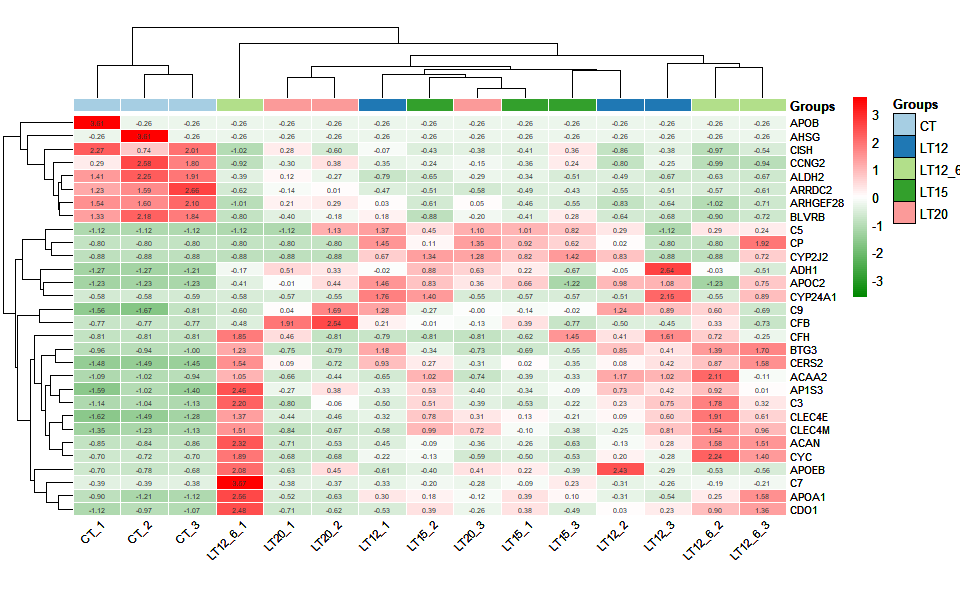
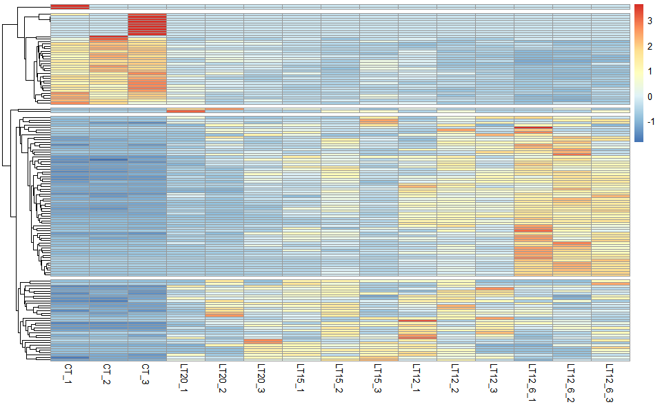
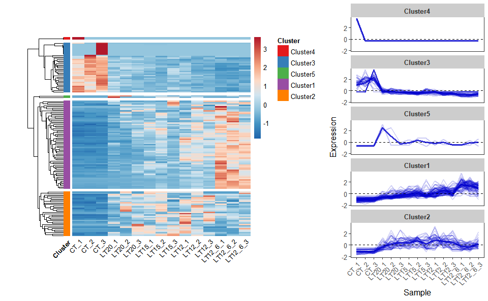
# ?TOmicsVis::network_plotInput Data: Dataframe: Shared DEGs of all paired comparisons in all samples expression dataframe of RNA-Seq. (1st-col: Genes, 2nd-col~: Samples).
Output Plot: Heatmap cluster plot for visualizing clustered gene expression data.
# 1. Load example datasets
data(gene_expression2)
head(gene_expression2)
#>   Genes  CT_1    CT_2  CT_3 LT20_1 LT20_2 LT20_3 LT15_1 LT15_2 LT15_3 LT12_1
#> 1 ACAA2 24.50   39.83 55.38 114.11 159.32  96.88 169.56 464.84 182.66 116.08
#> 2  ACAN 14.97   18.71 10.30  71.23 142.67 213.54 253.15 320.80 104.15 174.02
#> 3  ADH1  1.54    1.56  2.04  14.95  13.60  15.87  12.80  17.74   6.06  10.97
#> 4  AHSG  0.00 1911.99  0.00   0.00   0.00   0.00   0.00   0.00   0.00   0.00
#> 5 ALDH2  2.07    2.86  2.54   0.85   0.49   0.47   0.42   0.13   0.26   0.00
#> 6 AP1S3  6.62   14.59  9.30  24.90  33.94  23.19  24.00  36.08  27.40  24.06
#>   LT12_2 LT12_3 LT12_6_1 LT12_6_2 LT12_6_3
#> 1 497.29 464.48   471.43   693.62   229.77
#> 2 305.81 469.48  1291.90   991.90   966.77
#> 3  10.71  30.95     9.84    10.91     7.28
#> 4   0.00   0.00     0.00     0.00     0.00
#> 5   0.28   0.11     0.37     0.15     0.11
#> 6  38.74  34.54    62.72    41.36    28.75

# 2. Run network_plot plot function
heatmap_cluster(
  data = gene_expression2,
  dist_method = "euclidean",
  hc_method = "average",
  k_num = 5,
  show_rownames = FALSE,
  palette = "RdBu",
  cluster_pal = "Set1",
  border_color = "#ffffff",
  angle_col = 45,
  label_size = 10,
  base_size = 12,
  line_color = "#0000cd",
  line_alpha = 0.2,
  summary_color = "#0000cd",
  summary_alpha = 0.8
)
#> Using Cluster, gene as id variables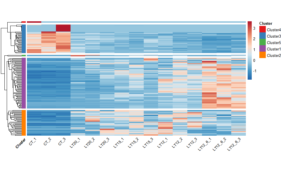
Get help using command ?TOmicsVis::heatmap_cluster or
reference page https://benben-miao.github.io/TOmicsVis/reference/heatmap_cluster.html.
# Get help with command in R console.
# ?TOmicsVis::heatmap_clusterInput Data: Dataframe: GO and KEGG annotation of background genes (1st-col: Genes, 2nd-col: biological_process, 3rd-col: cellular_component, 4th-col: molecular_function, 5th-col: kegg_pathway).
Output Table: GO enrichment analysis based on GO annotation results (None/Exist Reference Genome).
# 1. Load example datasets
data(gene_go_kegg)
head(gene_go_kegg)
#>        Genes
#> 1        FN1
#> 2 14-3-3ZETA
#> 3       A1I3
#> 4        A2M
#> 5       AARS
#> 6       ABAT
#>                                                                                                 biological_process
#> 1 GO:0003181(atrioventricular valve morphogenesis);GO:0003128(heart field specification);GO:0001756(somitogenesis)
#> 2                                                                                                             <NA>
#> 3                                                                                                             <NA>
#> 4                                                                                                             <NA>
#> 5                                                                           GO:0006419(alanyl-tRNA aminoacylation)
#> 6                                                            GO:0009448(gamma-aminobutyric acid metabolic process)
#>                 cellular_component
#> 1 GO:0005576(extracellular region)
#> 2                             <NA>
#> 3  GO:0005615(extracellular space)
#> 4  GO:0005615(extracellular space)
#> 5            GO:0005737(cytoplasm)
#> 6                             <NA>
#>                                                                                                       molecular_function
#> 1                                                                                                                   <NA>
#> 2                                                                            GO:0019904(protein domain specific binding)
#> 3                                                                           GO:0004866(endopeptidase inhibitor activity)
#> 4                                                                           GO:0004866(endopeptidase inhibitor activity)
#> 5 GO:0004813(alanine-tRNA ligase activity);GO:0005524(ATP binding);GO:0000049(tRNA binding);GO:0008270(zinc ion binding)
#> 6                              GO:0003867(4-aminobutyrate transaminase activity);GO:0030170(pyridoxal phosphate binding)
#>                                                                                                                                                                                                                                kegg_pathway
#> 1                                                                                                   ko04810(Regulation of actin cytoskeleton);ko04510(Focal adhesion);ko04151(PI3K-Akt signaling pathway);ko04512(ECM-receptor interaction)
#> 2 ko04110(Cell cycle);ko04114(Oocyte meiosis);ko04390(Hippo signaling pathway);ko04391(Hippo signaling pathway -fly);ko04013(MAPK signaling pathway - fly);ko04151(PI3K-Akt signaling pathway);ko04212(Longevity regulating pathway - worm)
#> 3                                                                                                                                                                                              ko04610(Complement and coagulation cascades)
#> 4                                                                                                                                                                                              ko04610(Complement and coagulation cascades)
#> 5                                                                                                                                                                                                      ko00970(Aminoacyl-tRNA biosynthesis)
#> 6         ko00250(Alanine, aspartate and glutamate metabolism);ko00280(Valine, leucine and isoleucine degradation);ko00650(Butanoate metabolism);ko00640(Propanoate metabolism);ko00410(beta-Alanine metabolism);ko04727(GABAergic synapse)

# 2. Run go_enrich analysis function
res <- go_enrich(
  go_anno = gene_go_kegg[,-5],
  degs_list = gene_go_kegg[100:200,1],
  padjust_method = "fdr",
  pvalue_cutoff = 0.05,
  qvalue_cutoff = 0.05
)
head(res)
#>           ID           ontology
#> 1 GO:0000221 cellular component
#> 2 GO:0000275 cellular component
#> 3 GO:0000276 cellular component
#> 4 GO:0000398 biological process
#> 5 GO:0000774 molecular function
#> 6 GO:0001671 molecular function
#>                                                                 Description
#> 1                     vacuolar proton-transporting V-type ATPase, V1 domain
#> 2  mitochondrial proton-transporting ATP synthase complex, catalytic core F
#> 3 mitochondrial proton-transporting ATP synthase complex, coupling factor F
#> 4                                            mRNA splicing, via spliceosome
#> 5                                adenyl-nucleotide exchange factor activity
#> 6                                                 ATPase activator activity
#>   GeneRatio BgRatio       pvalue     p.adjust       qvalue
#> 1     1/101  1/1279 7.896794e-02 1.110997e-01 9.458955e-02
#> 2     1/101  1/1279 7.896794e-02 1.110997e-01 9.458955e-02
#> 3     6/101  6/1279 2.109128e-07 1.075656e-05 9.158058e-06
#> 4     1/101 14/1279 6.858207e-01 7.363549e-01 6.269275e-01
#> 5     1/101  1/1279 7.896794e-02 1.110997e-01 9.458955e-02
#> 6     1/101  1/1279 7.896794e-02 1.110997e-01 9.458955e-02
#>                                       geneID Count
#> 1                                    ATP6V1H     1
#> 2                                    ATP5F1E     1
#> 3 ATP5MC1/ATP5ME/ATP5MG/ATP5PB/ATP5PD/ATP5PF     6
#> 4                                      CDC40     1
#> 5                                       BAG2     1
#> 6                                     ATP1B1     1
Get help using command ?TOmicsVis::go_enrich or
reference page https://benben-miao.github.io/TOmicsVis/reference/go_enrich.html.
# Get help with command in R console.
# ?TOmicsVis::go_enrichInput Data: Dataframe: GO and KEGG annotation of background genes (1st-col: Genes, 2nd-col: biological_process, 3rd-col: cellular_component, 4th-col: molecular_function, 5th-col: kegg_pathway).
Output Plot: GO enrichment analysis and stat plot (None/Exist Reference Genome).
# 1. Load example datasets
data(gene_go_kegg)

# 2. Run go_enrich_stat analysis function
go_enrich_stat(
  go_anno = gene_go_kegg[,-5],
  degs_list = gene_go_kegg[100:200,1],
  padjust_method = "fdr",
  pvalue_cutoff = 0.05,
  qvalue_cutoff = 0.05,
  max_go_item = 15,
  strip_fill = "#CDCDCD",
  xtext_angle = 45,
  sci_fill_color = "Sci_AAAS",
  sci_fill_alpha = 0.8,
  ggTheme = "theme_light"
)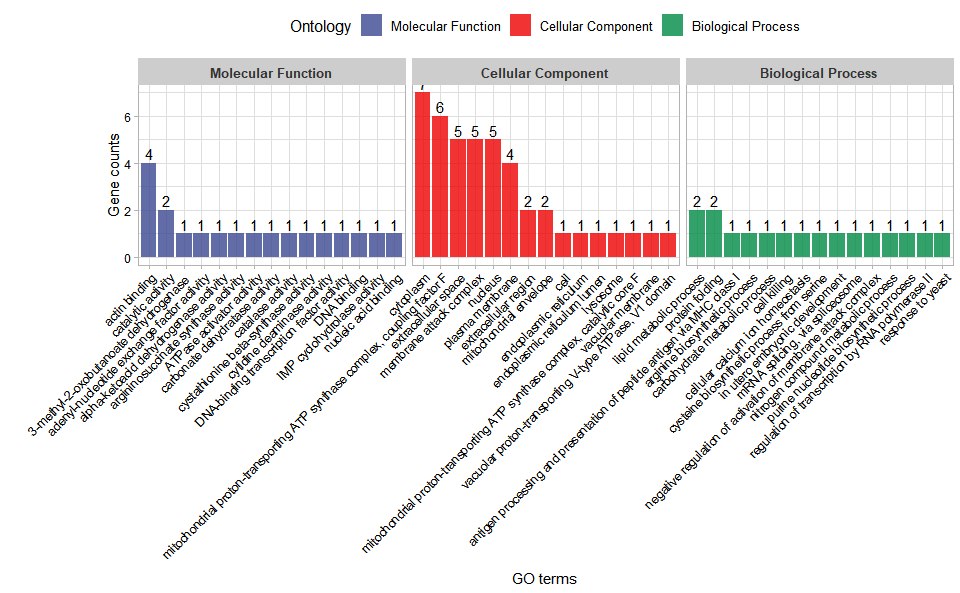
Get help using command ?TOmicsVis::go_enrich_stat or
reference page https://benben-miao.github.io/TOmicsVis/reference/go_enrich_stat.html.
# Get help with command in R console.
# ?TOmicsVis::go_enrich_statInput Data: Dataframe: GO and KEGG annotation of background genes (1st-col: Genes, 2nd-col: biological_process, 3rd-col: cellular_component, 4th-col: molecular_function, 5th-col: kegg_pathway).
Output Plot: GO enrichment analysis and bar plot (None/Exist Reference Genome).
# 1. Load example datasets
data(gene_go_kegg)

# 2. Run go_enrich_bar analysis function
go_enrich_bar(
  go_anno = gene_go_kegg[,-5],
  degs_list = gene_go_kegg[100:200,1],
  padjust_method = "fdr",
  pvalue_cutoff = 0.05,
  qvalue_cutoff = 0.05,
  sign_by = "p.adjust",
  category_num = 30,
  font_size = 12,
  low_color = "#ff0000aa",
  high_color = "#008800aa",
  ggTheme = "theme_light"
)
#> Scale for fill is already present.
#> Adding another scale for fill, which will replace the existing scale.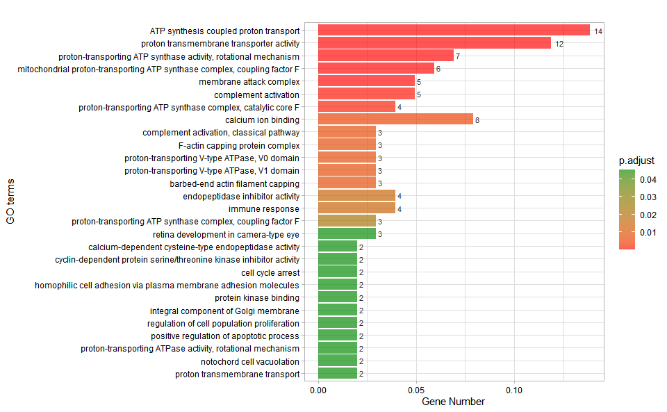
Get help using command ?TOmicsVis::go_enrich_bar or
reference page https://benben-miao.github.io/TOmicsVis/reference/go_enrich_bar.html.
# Get help with command in R console.
# ?TOmicsVis::go_enrich_barInput Data: Dataframe: GO and KEGG annotation of background genes (1st-col: Genes, 2nd-col: biological_process, 3rd-col: cellular_component, 4th-col: molecular_function, 5th-col: kegg_pathway).
Output Plot: GO enrichment analysis and dot plot (None/Exist Reference Genome).
# 1. Load example datasets
data(gene_go_kegg)

# 2. Run go_enrich_dot analysis function
go_enrich_dot(
  go_anno = gene_go_kegg[,-5],
  degs_list = gene_go_kegg[100:200,1],
  padjust_method = "fdr",
  pvalue_cutoff = 0.05,
  qvalue_cutoff = 0.05,
  sign_by = "p.adjust",
  category_num = 30,
  font_size = 12,
  low_color = "#ff0000aa",
  high_color = "#008800aa",
  ggTheme = "theme_light"
)
#> Scale for colour is already present.
#> Adding another scale for colour, which will replace the existing scale.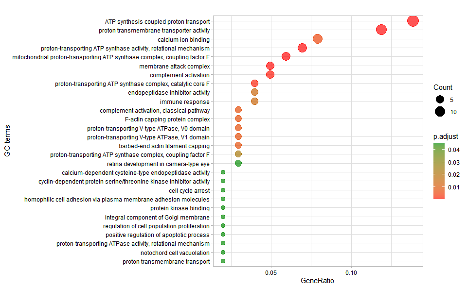
Get help using command ?TOmicsVis::go_enrich_dot or
reference page https://benben-miao.github.io/TOmicsVis/reference/go_enrich_dot.html.
# Get help with command in R console.
# ?TOmicsVis::go_enrich_dotInput Data: Dataframe: GO and KEGG annotation of background genes (1st-col: Genes, 2nd-col: biological_process, 3rd-col: cellular_component, 4th-col: molecular_function, 5th-col: kegg_pathway).
Output Plot: GO enrichment analysis and net plot (None/Exist Reference Genome).
# 1. Load example datasets
data(gene_go_kegg)

# 2. Run go_enrich_net analysis function
go_enrich_net(
  go_anno = gene_go_kegg[,-5],
  degs_list = gene_go_kegg[100:200,1],
  padjust_method = "fdr",
  pvalue_cutoff = 0.05,
  qvalue_cutoff = 0.05,
  category_num = 20,
  net_layout = "circle",
  net_circular = TRUE,
  low_color = "#ff0000aa",
  high_color = "#008800aa"
)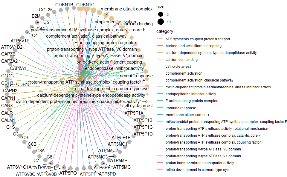
Get help using command ?TOmicsVis::go_enrich_net or
reference page https://benben-miao.github.io/TOmicsVis/reference/go_enrich_net.html.
# Get help with command in R console.
# ?TOmicsVis::go_enrich_netInput Data: Dataframe: GO and KEGG annotation of background genes (1st-col: Genes, 2nd-col: biological_process, 3rd-col: cellular_component, 4th-col: molecular_function, 5th-col: kegg_pathway).
Output Plot: GO enrichment analysis based on GO annotation results (None/Exist Reference Genome).
# 1. Load example datasets
data(gene_go_kegg)
head(gene_go_kegg)
#>        Genes
#> 1        FN1
#> 2 14-3-3ZETA
#> 3       A1I3
#> 4        A2M
#> 5       AARS
#> 6       ABAT
#>                                                                                                 biological_process
#> 1 GO:0003181(atrioventricular valve morphogenesis);GO:0003128(heart field specification);GO:0001756(somitogenesis)
#> 2                                                                                                             <NA>
#> 3                                                                                                             <NA>
#> 4                                                                                                             <NA>
#> 5                                                                           GO:0006419(alanyl-tRNA aminoacylation)
#> 6                                                            GO:0009448(gamma-aminobutyric acid metabolic process)
#>                 cellular_component
#> 1 GO:0005576(extracellular region)
#> 2                             <NA>
#> 3  GO:0005615(extracellular space)
#> 4  GO:0005615(extracellular space)
#> 5            GO:0005737(cytoplasm)
#> 6                             <NA>
#>                                                                                                       molecular_function
#> 1                                                                                                                   <NA>
#> 2                                                                            GO:0019904(protein domain specific binding)
#> 3                                                                           GO:0004866(endopeptidase inhibitor activity)
#> 4                                                                           GO:0004866(endopeptidase inhibitor activity)
#> 5 GO:0004813(alanine-tRNA ligase activity);GO:0005524(ATP binding);GO:0000049(tRNA binding);GO:0008270(zinc ion binding)
#> 6                              GO:0003867(4-aminobutyrate transaminase activity);GO:0030170(pyridoxal phosphate binding)
#>                                                                                                                                                                                                                                kegg_pathway
#> 1                                                                                                   ko04810(Regulation of actin cytoskeleton);ko04510(Focal adhesion);ko04151(PI3K-Akt signaling pathway);ko04512(ECM-receptor interaction)
#> 2 ko04110(Cell cycle);ko04114(Oocyte meiosis);ko04390(Hippo signaling pathway);ko04391(Hippo signaling pathway -fly);ko04013(MAPK signaling pathway - fly);ko04151(PI3K-Akt signaling pathway);ko04212(Longevity regulating pathway - worm)
#> 3                                                                                                                                                                                              ko04610(Complement and coagulation cascades)
#> 4                                                                                                                                                                                              ko04610(Complement and coagulation cascades)
#> 5                                                                                                                                                                                                      ko00970(Aminoacyl-tRNA biosynthesis)
#> 6         ko00250(Alanine, aspartate and glutamate metabolism);ko00280(Valine, leucine and isoleucine degradation);ko00650(Butanoate metabolism);ko00640(Propanoate metabolism);ko00410(beta-Alanine metabolism);ko04727(GABAergic synapse)

# 2. Run go_enrich analysis function
res <- kegg_enrich(
  kegg_anno = gene_go_kegg[,c(1,5)],
  degs_list = gene_go_kegg[100:200,1],
  padjust_method = "fdr",
  pvalue_cutoff = 0.05,
  qvalue_cutoff = 0.05
)
head(res)
#>              ID                         Description GeneRatio BgRatio
#> ko04966 ko04966      Collecting duct acid secretion     7/101  7/1279
#> ko00190 ko00190           Oxidative phosphorylation    23/101 88/1279
#> ko04721 ko04721              Synaptic vesicle cycle     8/101 13/1279
#> ko04610 ko04610 Complement and coagulation cascades    13/101 43/1279
#> ko04145 ko04145                           Phagosome    11/101 33/1279
#> ko04971 ko04971              Gastric acid secretion     4/101  4/1279
#>               pvalue     p.adjust       qvalue
#> ko04966 1.573976e-08 2.030430e-06 1.723090e-06
#> ko00190 5.232645e-08 3.375056e-06 2.864185e-06
#> ko04721 1.069634e-06 4.599427e-05 3.903227e-05
#> ko04610 1.078094e-05 3.476853e-04 2.950573e-04
#> ko04145 1.941460e-05 5.008968e-04 4.250776e-04
#> ko04971 3.679084e-05 7.910030e-04 6.712714e-04
#>                                                                                                                                                                                        geneID
#> ko04966                                                                                                                              ATP6V0C/ATP6V0E1/ATP6V1B2/ATP6V1C1A/ATP6V1F/ATP6V1G1/CA1
#> ko00190 ATP5F1A/ATP5F1B/ATP5F1C/ATP5F1D/ATP5F1E/ATP5MC1/ATP5MC2/ATP5MC3/ATP5ME/ATP5MF/ATP5MG/ATP5PB/ATP5PD/ATP5PF/ATP5PO/ATP6V0B/ATP6V0C/ATP6V0E1/ATP6V1B2/ATP6V1C1A/ATP6V1F/ATP6V1G1/ATP6V1H
#> ko04721                                                                                                                  ATP6V0B/ATP6V0C/ATP6V0E1/ATP6V1B2/ATP6V1C1A/ATP6V1F/ATP6V1G1/ATP6V1H
#> ko04610                                                                                                                                       C1QC/C1S/C3/C4/C4A/C5/C6/C7/C8A/C8B/C8G/C9/CD59
#> ko04145                                                                                                     ATP6V0B/ATP6V0C/ATP6V0E1/ATP6V1B2/ATP6V1C1A/ATP6V1F/ATP6V1G1/ATP6V1H/C3/CALR/CANX
#> ko04971                                                                                                                                                               ATP1B1/CA1/CALM1/CAMK2D
#>         Count
#> ko04966     7
#> ko00190    23
#> ko04721     8
#> ko04610    13
#> ko04145    11
#> ko04971     4
Get help using command ?TOmicsVis::kegg_enrich or
reference page https://benben-miao.github.io/TOmicsVis/reference/kegg_enrich.html.
# Get help with command in R console.
# ?TOmicsVis::kegg_enrichInput Data: Dataframe: GO and KEGG annotation of background genes (1st-col: Genes, 2nd-col: biological_process, 3rd-col: cellular_component, 4th-col: molecular_function, 5th-col: kegg_pathway).
Output Plot: KEGG enrichment analysis and bar plot (None/Exist Reference Genome).
# 1. Load example datasets
data(gene_go_kegg)

# 2. Run kegg_enrich_bar analysis function
kegg_enrich_bar(
  kegg_anno = gene_go_kegg[,c(1,5)],
  degs_list = gene_go_kegg[100:200,1],
  padjust_method = "fdr",
  pvalue_cutoff = 0.05,
  qvalue_cutoff = 0.05,
  sign_by = "p.adjust",
  category_num = 30,
  font_size = 12,
  low_color = "#ff0000aa",
  high_color = "#008800aa",
  ggTheme = "theme_light"
)
#> Scale for fill is already present.
#> Adding another scale for fill, which will replace the existing scale.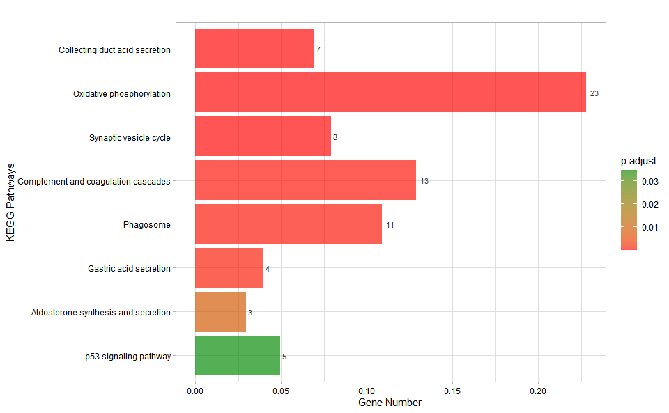
Get help using command ?TOmicsVis::kegg_enrich_bar or
reference page https://benben-miao.github.io/TOmicsVis/reference/kegg_enrich_bar.html.
# Get help with command in R console.
# ?TOmicsVis::kegg_enrich_barInput Data: Dataframe: GO and KEGG annotation of background genes (1st-col: Genes, 2nd-col: biological_process, 3rd-col: cellular_component, 4th-col: molecular_function, 5th-col: kegg_pathway).
Output Plot: KEGG enrichment analysis and dot plot (None/Exist Reference Genome).
# 1. Load example datasets
data(gene_go_kegg)

# 2. Run kegg_enrich_dot analysis function
kegg_enrich_dot(
  kegg_anno = gene_go_kegg[,c(1,5)],
  degs_list = gene_go_kegg[100:200,1],
  padjust_method = "fdr",
  pvalue_cutoff = 0.05,
  qvalue_cutoff = 0.05,
  sign_by = "p.adjust",
  category_num = 30,
  font_size = 12,
  low_color = "#ff0000aa",
  high_color = "#008800aa",
  ggTheme = "theme_light"
)
#> Scale for colour is already present.
#> Adding another scale for colour, which will replace the existing scale.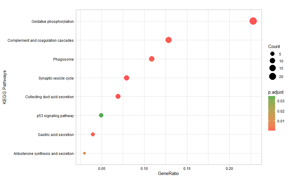
Get help using command ?TOmicsVis::kegg_enrich_dot or
reference page https://benben-miao.github.io/TOmicsVis/reference/kegg_enrich_dot.html.
# Get help with command in R console.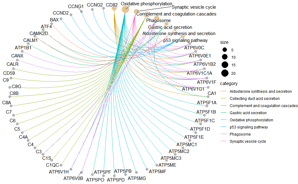
# ?TOmicsVis::kegg_enrich_dotInput Data: Dataframe: GO and KEGG annotation of background genes (1st-col: Genes, 2nd-col: biological_process, 3rd-col: cellular_component, 4th-col: molecular_function, 5th-col: kegg_pathway).
Output Plot: KEGG enrichment analysis and net plot (None/Exist Reference Genome).
# 1. Load example datasets
data(gene_go_kegg)

# 2. Run kegg_enrich_net analysis function
kegg_enrich_net(
  kegg_anno = gene_go_kegg[,c(1,5)],
  degs_list = gene_go_kegg[100:200,1],
  padjust_method = "fdr",
  pvalue_cutoff = 0.05,
  qvalue_cutoff = 0.05,
  category_num = 20,
  net_layout = "circle",
  net_circular = TRUE,
  low_color = "#ff0000aa",
  high_color = "#008800aa"
)
Get help using command ?TOmicsVis::kegg_enrich_net or
reference page https://benben-miao.github.io/TOmicsVis/reference/kegg_enrich_net.html.
# Get help with command in R console.
# ?TOmicsVis::kegg_enrich_netInput Data: Dataframe: GO and KEGG annotation of background genes (1st-col: Genes, 2nd-col: biological_process, 3rd-col: cellular_component, 4th-col: molecular_function, 5th-col: kegg_pathway).
Output Table: Table split used for splitting a grouped column to multiple columns.
# 1. Load example datasets
data(gene_go_kegg2)
head(gene_go_kegg2)
#>        Genes
#> 1        FN1
#> 2 14-3-3ZETA
#> 3       A1I3
#> 4        A2M
#> 5       AARS
#> 6       ABAT
#>                                                                                                                                                                                                                                kegg_pathway
#> 1                                                                                                   ko04810(Regulation of actin cytoskeleton);ko04510(Focal adhesion);ko04151(PI3K-Akt signaling pathway);ko04512(ECM-receptor interaction)
#> 2 ko04110(Cell cycle);ko04114(Oocyte meiosis);ko04390(Hippo signaling pathway);ko04391(Hippo signaling pathway -fly);ko04013(MAPK signaling pathway - fly);ko04151(PI3K-Akt signaling pathway);ko04212(Longevity regulating pathway - worm)
#> 3                                                                                                                                                                                              ko04610(Complement and coagulation cascades)
#> 4                                                                                                                                                                                              ko04610(Complement and coagulation cascades)
#> 5                                                                                                                                                                                                      ko00970(Aminoacyl-tRNA biosynthesis)
#> 6         ko00250(Alanine, aspartate and glutamate metabolism);ko00280(Valine, leucine and isoleucine degradation);ko00650(Butanoate metabolism);ko00640(Propanoate metabolism);ko00410(beta-Alanine metabolism);ko04727(GABAergic synapse)
#>          go_category
#> 1 biological_process
#> 2 biological_process
#> 3 biological_process
#> 4 biological_process
#> 5 biological_process
#> 6 biological_process
#>                                                                                                            go_term
#> 1 GO:0003181(atrioventricular valve morphogenesis);GO:0003128(heart field specification);GO:0001756(somitogenesis)
#> 2                                                                                                             <NA>
#> 3                                                                                                             <NA>
#> 4                                                                                                             <NA>
#> 5                                                                           GO:0006419(alanyl-tRNA aminoacylation)
#> 6                                                            GO:0009448(gamma-aminobutyric acid metabolic process)

# 2. Run table_split function
res <- table_split(
  data = gene_go_kegg2,
  grouped_var = "go_category",
  value_var = "go_term",
  miss_drop = TRUE
)
head(res)
#>        Genes
#> 1 14-3-3ZETA
#> 2       A1I3
#> 3        A2M
#> 4       AARS
#> 5       ABAT
#> 6      ABCB7
#>                                                                                                                                                                                                                                kegg_pathway
#> 1 ko04110(Cell cycle);ko04114(Oocyte meiosis);ko04390(Hippo signaling pathway);ko04391(Hippo signaling pathway -fly);ko04013(MAPK signaling pathway - fly);ko04151(PI3K-Akt signaling pathway);ko04212(Longevity regulating pathway - worm)
#> 2                                                                                                                                                                                              ko04610(Complement and coagulation cascades)
#> 3                                                                                                                                                                                              ko04610(Complement and coagulation cascades)
#> 4                                                                                                                                                                                                      ko00970(Aminoacyl-tRNA biosynthesis)
#> 5         ko00250(Alanine, aspartate and glutamate metabolism);ko00280(Valine, leucine and isoleucine degradation);ko00650(Butanoate metabolism);ko00640(Propanoate metabolism);ko00410(beta-Alanine metabolism);ko04727(GABAergic synapse)
#> 6                                                                                                                                                                                                                 ko02010(ABC transporters)
#>                                      biological_process
#> 1                                                  <NA>
#> 2                                                  <NA>
#> 3                                                  <NA>
#> 4                GO:0006419(alanyl-tRNA aminoacylation)
#> 5 GO:0009448(gamma-aminobutyric acid metabolic process)
#> 6                                                  <NA>
#>                           cellular_component
#> 1                                       <NA>
#> 2            GO:0005615(extracellular space)
#> 3            GO:0005615(extracellular space)
#> 4                      GO:0005737(cytoplasm)
#> 5                                       <NA>
#> 6 GO:0016021(integral component of membrane)
#>                                                                                                       molecular_function
#> 1                                                                            GO:0019904(protein domain specific binding)
#> 2                                                                           GO:0004866(endopeptidase inhibitor activity)
#> 3                                                                           GO:0004866(endopeptidase inhibitor activity)
#> 4 GO:0004813(alanine-tRNA ligase activity);GO:0005524(ATP binding);GO:0000049(tRNA binding);GO:0008270(zinc ion binding)
#> 5                              GO:0003867(4-aminobutyrate transaminase activity);GO:0030170(pyridoxal phosphate binding)
#> 6      GO:0005524(ATP binding);GO:0016887(ATPase activity);GO:0042626(ATPase-coupled transmembrane transporter activity)
Get help using command ?TOmicsVis::table_split or
reference page https://benben-miao.github.io/TOmicsVis/reference/table_split.html.
# Get help with command in R console.
# ?TOmicsVis::table_splitInput Data: Dataframe: GO and KEGG annotation of background genes (1st-col: Genes, 2nd-col: biological_process, 3rd-col: cellular_component, 4th-col: molecular_function, 5th-col: kegg_pathway).
Output Table: Table merge used to merge multiple variables to on variable.
# 1. Load example datasets
data(gene_go_kegg)
head(gene_go_kegg)
#>        Genes
#> 1        FN1
#> 2 14-3-3ZETA
#> 3       A1I3
#> 4        A2M
#> 5       AARS
#> 6       ABAT
#>                                                                                                 biological_process
#> 1 GO:0003181(atrioventricular valve morphogenesis);GO:0003128(heart field specification);GO:0001756(somitogenesis)
#> 2                                                                                                             <NA>
#> 3                                                                                                             <NA>
#> 4                                                                                                             <NA>
#> 5                                                                           GO:0006419(alanyl-tRNA aminoacylation)
#> 6                                                            GO:0009448(gamma-aminobutyric acid metabolic process)
#>                 cellular_component
#> 1 GO:0005576(extracellular region)
#> 2                             <NA>
#> 3  GO:0005615(extracellular space)
#> 4  GO:0005615(extracellular space)
#> 5            GO:0005737(cytoplasm)
#> 6                             <NA>
#>                                                                                                       molecular_function
#> 1                                                                                                                   <NA>
#> 2                                                                            GO:0019904(protein domain specific binding)
#> 3                                                                           GO:0004866(endopeptidase inhibitor activity)
#> 4                                                                           GO:0004866(endopeptidase inhibitor activity)
#> 5 GO:0004813(alanine-tRNA ligase activity);GO:0005524(ATP binding);GO:0000049(tRNA binding);GO:0008270(zinc ion binding)
#> 6                              GO:0003867(4-aminobutyrate transaminase activity);GO:0030170(pyridoxal phosphate binding)
#>                                                                                                                                                                                                                                kegg_pathway
#> 1                                                                                                   ko04810(Regulation of actin cytoskeleton);ko04510(Focal adhesion);ko04151(PI3K-Akt signaling pathway);ko04512(ECM-receptor interaction)
#> 2 ko04110(Cell cycle);ko04114(Oocyte meiosis);ko04390(Hippo signaling pathway);ko04391(Hippo signaling pathway -fly);ko04013(MAPK signaling pathway - fly);ko04151(PI3K-Akt signaling pathway);ko04212(Longevity regulating pathway - worm)
#> 3                                                                                                                                                                                              ko04610(Complement and coagulation cascades)
#> 4                                                                                                                                                                                              ko04610(Complement and coagulation cascades)
#> 5                                                                                                                                                                                                      ko00970(Aminoacyl-tRNA biosynthesis)
#> 6         ko00250(Alanine, aspartate and glutamate metabolism);ko00280(Valine, leucine and isoleucine degradation);ko00650(Butanoate metabolism);ko00640(Propanoate metabolism);ko00410(beta-Alanine metabolism);ko04727(GABAergic synapse)

# 2. Run function
res <- table_merge(
  data = gene_go_kegg,
  merge_vars = c("biological_process", "cellular_component", "molecular_function"),
  new_var = "go_category",
  new_value = "go_term",
  na_remove = FALSE
)
head(res)
#>        Genes
#> 1        FN1
#> 2 14-3-3ZETA
#> 3       A1I3
#> 4        A2M
#> 5       AARS
#> 6       ABAT
#>                                                                                                                                                                                                                                kegg_pathway
#> 1                                                                                                   ko04810(Regulation of actin cytoskeleton);ko04510(Focal adhesion);ko04151(PI3K-Akt signaling pathway);ko04512(ECM-receptor interaction)
#> 2 ko04110(Cell cycle);ko04114(Oocyte meiosis);ko04390(Hippo signaling pathway);ko04391(Hippo signaling pathway -fly);ko04013(MAPK signaling pathway - fly);ko04151(PI3K-Akt signaling pathway);ko04212(Longevity regulating pathway - worm)
#> 3                                                                                                                                                                                              ko04610(Complement and coagulation cascades)
#> 4                                                                                                                                                                                              ko04610(Complement and coagulation cascades)
#> 5                                                                                                                                                                                                      ko00970(Aminoacyl-tRNA biosynthesis)
#> 6         ko00250(Alanine, aspartate and glutamate metabolism);ko00280(Valine, leucine and isoleucine degradation);ko00650(Butanoate metabolism);ko00640(Propanoate metabolism);ko00410(beta-Alanine metabolism);ko04727(GABAergic synapse)
#>          go_category
#> 1 biological_process
#> 2 biological_process
#> 3 biological_process
#> 4 biological_process
#> 5 biological_process
#> 6 biological_process
#>                                                                                                            go_term
#> 1 GO:0003181(atrioventricular valve morphogenesis);GO:0003128(heart field specification);GO:0001756(somitogenesis)
#> 2                                                                                                             <NA>
#> 3                                                                                                             <NA>
#> 4                                                                                                             <NA>
#> 5                                                                           GO:0006419(alanyl-tRNA aminoacylation)
#> 6                                                            GO:0009448(gamma-aminobutyric acid metabolic process)
Get help using command ?TOmicsVis::table_merge or
reference page https://benben-miao.github.io/TOmicsVis/reference/table_merge.html.
# Get help with command in R console.
# ?TOmicsVis::table_mergeInput Data: Dataframe: GO and KEGG annotation of background genes (1st-col: Genes, 2nd-col: biological_process, 3rd-col: cellular_component, 4th-col: molecular_function, 5th-col: kegg_pathway).
Output Table: Table filter used to filter row by column condition.
# 1. Load example datasets
data(traits_sex)
head(traits_sex)
#>   Value Traits    Sex
#> 1 36.74 Weight Female
#> 2 38.54 Weight Female
#> 3 44.91 Weight Female
#> 4 43.53 Weight Female
#> 5 39.03 Weight Female
#> 6 26.01 Weight Female

# 2. Run function
res <- table_filter(
    data = traits_sex,
    Sex == "Male" & Traits == "Weight" & Value > 40
    )
head(res)
#>   Value Traits  Sex
#> 1 48.06 Weight Male
#> 2 42.74 Weight Male
#> 3 45.25 Weight Male
#> 4 44.95 Weight Male
#> 5 43.21 Weight Male
#> 6 40.02 Weight Male
Get help using command ?TOmicsVis::table_filter or
reference page https://benben-miao.github.io/TOmicsVis/reference/table_filter.html.
# Get help with command in R console.
# ?TOmicsVis::table_filterInput Data1: Dataframe: Shared DEGs of all paired comparisons in all samples expression dataframe of RNA-Seq. (1st-col: Genes, 2nd-col~: Samples).
Input Data2: Dataframe: GO and KEGG annotation of background genes (1st-col: Genes, 2nd-col: biological_process, 3rd-col: cellular_component, 4th-col: molecular_function, 5th-col: kegg_pathway).
Output Plot: Table cross used to cross search and merge results in two tables.
# 1. Load example datasets
data(gene_expression2)
head(gene_expression2)
#>   Genes  CT_1    CT_2  CT_3 LT20_1 LT20_2 LT20_3 LT15_1 LT15_2 LT15_3 LT12_1
#> 1 ACAA2 24.50   39.83 55.38 114.11 159.32  96.88 169.56 464.84 182.66 116.08
#> 2  ACAN 14.97   18.71 10.30  71.23 142.67 213.54 253.15 320.80 104.15 174.02
#> 3  ADH1  1.54    1.56  2.04  14.95  13.60  15.87  12.80  17.74   6.06  10.97
#> 4  AHSG  0.00 1911.99  0.00   0.00   0.00   0.00   0.00   0.00   0.00   0.00
#> 5 ALDH2  2.07    2.86  2.54   0.85   0.49   0.47   0.42   0.13   0.26   0.00
#> 6 AP1S3  6.62   14.59  9.30  24.90  33.94  23.19  24.00  36.08  27.40  24.06
#>   LT12_2 LT12_3 LT12_6_1 LT12_6_2 LT12_6_3
#> 1 497.29 464.48   471.43   693.62   229.77
#> 2 305.81 469.48  1291.90   991.90   966.77
#> 3  10.71  30.95     9.84    10.91     7.28
#> 4   0.00   0.00     0.00     0.00     0.00
#> 5   0.28   0.11     0.37     0.15     0.11
#> 6  38.74  34.54    62.72    41.36    28.75

data(gene_go_kegg)
head(gene_go_kegg)
#>        Genes
#> 1        FN1
#> 2 14-3-3ZETA
#> 3       A1I3
#> 4        A2M
#> 5       AARS
#> 6       ABAT
#>                                                                                                 biological_process
#> 1 GO:0003181(atrioventricular valve morphogenesis);GO:0003128(heart field specification);GO:0001756(somitogenesis)
#> 2                                                                                                             <NA>
#> 3                                                                                                             <NA>
#> 4                                                                                                             <NA>
#> 5                                                                           GO:0006419(alanyl-tRNA aminoacylation)
#> 6                                                            GO:0009448(gamma-aminobutyric acid metabolic process)
#>                 cellular_component
#> 1 GO:0005576(extracellular region)
#> 2                             <NA>
#> 3  GO:0005615(extracellular space)
#> 4  GO:0005615(extracellular space)
#> 5            GO:0005737(cytoplasm)
#> 6                             <NA>
#>                                                                                                       molecular_function
#> 1                                                                                                                   <NA>
#> 2                                                                            GO:0019904(protein domain specific binding)
#> 3                                                                           GO:0004866(endopeptidase inhibitor activity)
#> 4                                                                           GO:0004866(endopeptidase inhibitor activity)
#> 5 GO:0004813(alanine-tRNA ligase activity);GO:0005524(ATP binding);GO:0000049(tRNA binding);GO:0008270(zinc ion binding)
#> 6                              GO:0003867(4-aminobutyrate transaminase activity);GO:0030170(pyridoxal phosphate binding)
#>                                                                                                                                                                                                                                kegg_pathway
#> 1                                                                                                   ko04810(Regulation of actin cytoskeleton);ko04510(Focal adhesion);ko04151(PI3K-Akt signaling pathway);ko04512(ECM-receptor interaction)
#> 2 ko04110(Cell cycle);ko04114(Oocyte meiosis);ko04390(Hippo signaling pathway);ko04391(Hippo signaling pathway -fly);ko04013(MAPK signaling pathway - fly);ko04151(PI3K-Akt signaling pathway);ko04212(Longevity regulating pathway - worm)
#> 3                                                                                                                                                                                              ko04610(Complement and coagulation cascades)
#> 4                                                                                                                                                                                              ko04610(Complement and coagulation cascades)
#> 5                                                                                                                                                                                                      ko00970(Aminoacyl-tRNA biosynthesis)
#> 6         ko00250(Alanine, aspartate and glutamate metabolism);ko00280(Valine, leucine and isoleucine degradation);ko00650(Butanoate metabolism);ko00640(Propanoate metabolism);ko00410(beta-Alanine metabolism);ko04727(GABAergic synapse)

# 2. Run function
res <- table_cross(
  data1 = gene_expression2,
  data2 = gene_go_kegg,
  inter_var = "Genes",
  left_index = TRUE,
  right_index = TRUE
)
head(res)
#>        Genes CT_1 CT_2 CT_3 LT20_1 LT20_2 LT20_3 LT15_1 LT15_2 LT15_3 LT12_1
#> 1 14-3-3ZETA   NA   NA   NA     NA     NA     NA     NA     NA     NA     NA
#> 2       A1I3   NA   NA   NA     NA     NA     NA     NA     NA     NA     NA
#> 3        A2M   NA   NA   NA     NA     NA     NA     NA     NA     NA     NA
#> 4       AARS   NA   NA   NA     NA     NA     NA     NA     NA     NA     NA
#> 5       ABAT   NA   NA   NA     NA     NA     NA     NA     NA     NA     NA
#> 6      ABCB7   NA   NA   NA     NA     NA     NA     NA     NA     NA     NA
#>   LT12_2 LT12_3 LT12_6_1 LT12_6_2 LT12_6_3
#> 1     NA     NA       NA       NA       NA
#> 2     NA     NA       NA       NA       NA
#> 3     NA     NA       NA       NA       NA
#> 4     NA     NA       NA       NA       NA
#> 5     NA     NA       NA       NA       NA
#> 6     NA     NA       NA       NA       NA
#>                                      biological_process
#> 1                                                  <NA>
#> 2                                                  <NA>
#> 3                                                  <NA>
#> 4                GO:0006419(alanyl-tRNA aminoacylation)
#> 5 GO:0009448(gamma-aminobutyric acid metabolic process)
#> 6                                                  <NA>
#>                           cellular_component
#> 1                                       <NA>
#> 2            GO:0005615(extracellular space)
#> 3            GO:0005615(extracellular space)
#> 4                      GO:0005737(cytoplasm)
#> 5                                       <NA>
#> 6 GO:0016021(integral component of membrane)
#>                                                                                                       molecular_function
#> 1                                                                            GO:0019904(protein domain specific binding)
#> 2                                                                           GO:0004866(endopeptidase inhibitor activity)
#> 3                                                                           GO:0004866(endopeptidase inhibitor activity)
#> 4 GO:0004813(alanine-tRNA ligase activity);GO:0005524(ATP binding);GO:0000049(tRNA binding);GO:0008270(zinc ion binding)
#> 5                              GO:0003867(4-aminobutyrate transaminase activity);GO:0030170(pyridoxal phosphate binding)
#> 6      GO:0005524(ATP binding);GO:0016887(ATPase activity);GO:0042626(ATPase-coupled transmembrane transporter activity)
#>                                                                                                                                                                                                                                kegg_pathway
#> 1 ko04110(Cell cycle);ko04114(Oocyte meiosis);ko04390(Hippo signaling pathway);ko04391(Hippo signaling pathway -fly);ko04013(MAPK signaling pathway - fly);ko04151(PI3K-Akt signaling pathway);ko04212(Longevity regulating pathway - worm)
#> 2                                                                                                                                                                                              ko04610(Complement and coagulation cascades)
#> 3                                                                                                                                                                                              ko04610(Complement and coagulation cascades)
#> 4                                                                                                                                                                                                      ko00970(Aminoacyl-tRNA biosynthesis)
#> 5         ko00250(Alanine, aspartate and glutamate metabolism);ko00280(Valine, leucine and isoleucine degradation);ko00650(Butanoate metabolism);ko00640(Propanoate metabolism);ko00410(beta-Alanine metabolism);ko04727(GABAergic synapse)
#> 6                                                                                                                                                                                                                 ko02010(ABC transporters)
Get help using command ?TOmicsVis::table_cross or
reference page https://benben-miao.github.io/TOmicsVis/reference/table_cross.html.
# Get help with command in R console.
# ?TOmicsVis::table_cross
These binaries (installable software) and packages are in development.
They may not be fully stable and should be used with caution. We make no claims about them.
Health stats visible at Monitor.