The hardware and bandwidth for this mirror is donated by dogado GmbH, the Webhosting and Full Service-Cloud Provider. Check out our Wordpress Tutorial.
If you wish to report a bug, or if you are interested in having us mirror your free-software or open-source project, please feel free to contact us at mirror[@]dogado.de.
![]()
The R package SppTrend provides a methodological
framework to analyse temporal changes in species occurrence patterns in
relation to spatial variables (longitude, latitude, and elevation) and
temperature. It is designed to support the development of explanatory
hypotheses on the effects of environmental change on species assemblages
by analysing opportunistically collected occurrence data that include
temporal and geographic information.
You can install the released version of SppTrend from CRAN:
install.packages("SppTrend")Alternatively, you can install the development version from GitHub:
install.packages("devtools")
library(devtools)
devtools::install_github("MarioMingarro/SppTrend")
library(SppTrend)SppTrend helps to characterise species responses to
environmental change by analysing historical occurrence data that
include:
Predictors - Sampling date (year, preferably month and year)
Responses - Geographic coordinates (latitude and longitude) and environmental variables (elevation and temperature).
The methodology assumes that observed species occurrences represent a temporal sequence of spatial and thermal responses to environmental change.
SppTrend provides a structured workflow for analyzing
these trends:
Exploratory diagnostic: Quickly visualize the
spatial distribution of occurrences and temporal temperature trends
within the area of presence using get_fast_info(), based on
NetCDF environmental data.
Environmental data integration (optional):
Enhance the occurrence records with environmental information using
functions like get_era5_tme() for temperature data or
get_elevation() for elevation.
Overall trend estimation: Estimate the average
temporal trend of selected response variables across all species using
overall_trend(). This trend serves as a baseline against
which individual species’ trends are compared.
Individual trend analysis: Estimate
specific-specific temporal trends for each response variable using
spp_trend(), enabling direct comparison between individual
species responses and the overall trend.
Ecological strategy classification: Classify
species into distinct spatial or thermal response categories based on
the direction and statistical significance of their species-specific
trends relative to the overall trend using
spp_strategy().
To utilize the package effectively, the input dataset must include the following information for each record:
species).lat) and Longitude
(lon). Note: Coordinates must be in the EPSG:4326
(WGS84) geographic coordinate reference system, which is the standard
for biodiversity occurrence data.year) is
required. Including month (month) is strongly recommended
to allow more detailed temporal analyses.Important
Ensure that the column names in your input dataset match the
default names expected by the SppTrend functions. These
default names are:
speciesyearmonthlonlattme
eleBefore starting the analysis, ensure you have the following components ready:
species, year, month,
lat, and lon..nc (NetCDF)
file to analyze temperature trends. See
get_era5_tme()..tif
(GeoTIFF) file for elevation analysis. See
get_elevation()readr, and
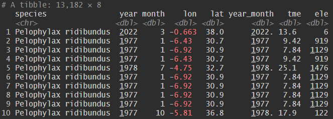
SppTrend.The following is an example using ranidae example from GBIF and selected in the exted (lon: -10 >= record <= 10 & lat: -40 >= record <= 40) and in dates (year >= 1950).
A total of 13,808 records of 15 different species.
ranidae <- readr::read_csv2(system.file("extdata", "example_ranidae.csv", package = "SppTrend"),
                    col_types = cols(year = col_double(),
                                     month = col_double(),
                                     lon = col_double(),
                                     lat = col_double()))
To capture intra-annual variations and treat time as a continuous
high-resolution variable, we combine year and
month into a single decimal predictor
(year_month). This transformation allows the models to use
a continuous variable representing the exact temporal position of each
record, providing a more nuanced analysis of temporal trends.
ranidae$year_month <- ranidae$year + ((ranidae$month - 1) / 12)
print(head(ranidae))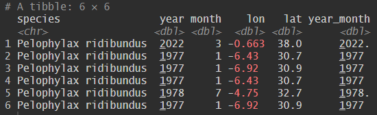
The get_fast_info() function provides a quick visual
diagnostic of the input data. It generates a map showing the spatial
distribution of occurrence records together with a time-series plot
derived from a NetCDF environmental dataste. Using the geographic
coordinates of the occurrence records, the function extracts the
complete climate time-series (from the earliest to the latest year
represented in the data) for the corresponding occupied cells. All
temperature values from occupied cells are then added annually to
estimate and visualise the overall temperature trend (including slope
and associated p-value). This diagnostic step allows users to quickly
assess the climate trajectory of the regions where the species have been
recorded and to evaluate whether sufficient temporal and environmental
variation is present for subsequent analyses.
Technical notes:
- See get_era5_tme()
nc_file <- "path/to/your/era5_data.nc"
info <- get_fast_info(ranidae, nc_file)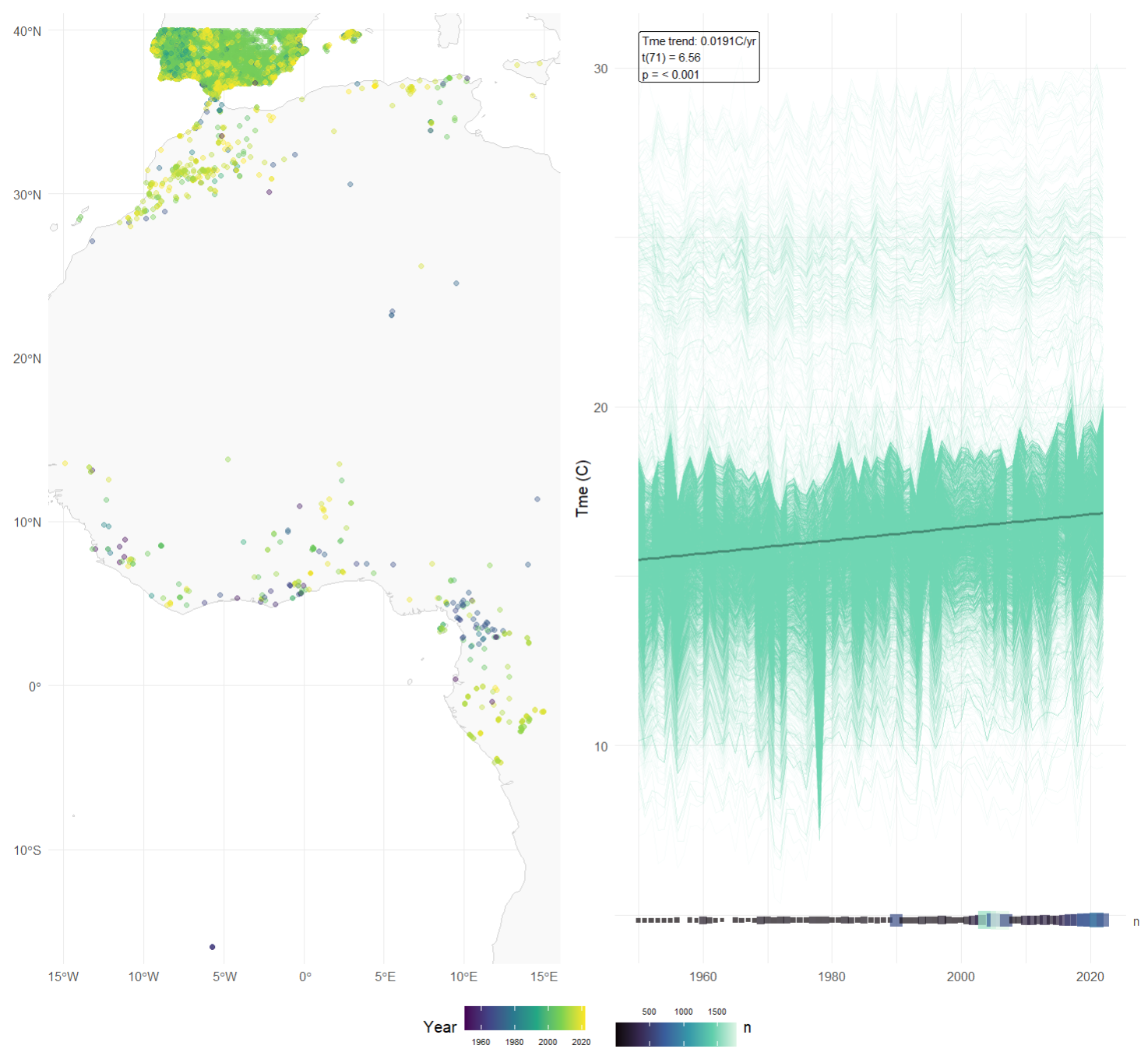
The SppTrend package provides functions to enhance
species occurrence records with relevant environmental information. At
present, it supports the integration of monthly temperature data and
elevation data associated with each occurrence.
ERA5 is the fifth-generation reanalysis dataset produced by the European Centre for Medium-Range Weather Forecasts (ECMWF), providing a globally consistent representation of atmospheric, land, and ocean conditions. If offers high spatial and temporal resolution climate data from 1940 to the present, making it a valuable and widely used resource for assessing the influence of climate on species distributions. Explore the ERA5-Land monthly averaged data from 1950 to present dataset on the Copernicus Climate Change Service (C3S) Climate Data Store (CDS) at: ERA5 Land monthly. For detailed information about the ERA5 dataset, please visit the ECMWF website.
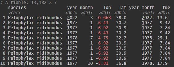
The SppTrend package provides the function
get_era5_tme() to incorporate ERA5-Land monthly climate
data. This function retrieves mean monthly air temperature values
associated with species occurrence records based on their geographic
coordinates (latitude and longitude) and sampling date (year and
month).
Technical notes:
- Temporal coverage: ERA5 data is available from 1950 to the present.
- Source: Download data from ERA5 Land monthly.
- Format: Files must be in .nc (NetCDF) format.
nc_file <- "path/to/your/era5_data.nc"
ranidae <- get_era5_tme(ranidae, nc_file)
print(head(ranidae))
Missing temperature data (NA) for 572 points. Removing records.
The get_elevation() function retrieves Digital Elevation
Model (DEM) values associated with species occurrence records, providing
information ont the elevation at which each species was observed. For
obtaining elevation data for species occurrences, this example utilizes
the WorldClim dataset (WorldClim).
However, users are encouraged to select alternative DEM sources
depending on the spatial resolution and geographic scope required for
their analysis. For instance, the EU-DEM
dataset offers high-resolution elevation data for Europe.
Technical notes:
- Format: DEM data must be in .tif format.
dem_file <- "path/to/your/dem.tif"
ranidae <- get_elevation(ranidae, dem_file)
print(head(ranidae))
Missing elevation data (NA) for 54 points. Removing records
The overall_trend() function calculates the overall
temporal trend (OT) of selected response variables across the entire
dataset. This trend integrates both environmental change and the
cumulative effects of sampling bias, and serves as a neutral reference
against which species-specific temporal trends are evaluated.
Technical notes:
Longitude (lon) values are transformed to a 0-360
range to ensure statistical consistency near the antimeridian.
A key feature of this function is its specialized handling of latitude. Because the Equator is set at 0, latitude values in the Southern Hemisphere are negative.
To ensure that a direction shift is interpreted consistently across the globe (where a negative increase in the South corresponds to a positive increase in the North), the function employs two complementary approaches:
- Hemispheric split: It divides the records based on their
location (lat < 0 for South and
lat > 0 for North) and performs separate
analyses for each.
- Global analysis: It performs an analysis using the complete
dataset (Global) by transforming all latitudes into
absolute values (abs(lat)). This allows for a unified
global trend estimation.
Note that this hemispheric division and absolute transformation logic
is applied exclusively to the latitude (lat) variable.
predictor <- "year_month"
responses <- c("lat", "lon", "ele", "tme")
overall_trend_result <- overall_trend(ranidae, predictor, responses)
print(head(overall_trend_result))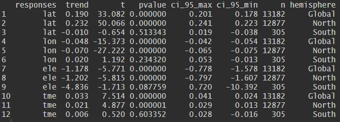
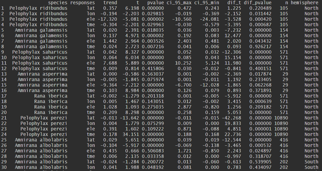
The spp_trend() function estimates the species-specific
temporal trends for each selected response variable and statistically
compares them with the overall temporal trend derived from the complete
dataset.
Technical notes:
It compares individual species’ trajectories against the OT using
the interaction term of the lm().
Longitude (lon) values are transformed to a 0-360
range to ensure statistical consistency near the antimeridian.
A key feature of this function is its specialized handling of latitude. Because the Equator is set at 0, latitude values in the Southern Hemisphere are negative.
To ensure that a direction shift is interpreted consistently across the globe (where a negative increase in the South corresponds to a positive increase in the North), the function employs two complementary approaches:
- Hemispheric split: It divides the records based on their
location (lat < 0 for South and
lat > 0 for North) and performs separate
analyses for each.
- Global analysis: It performs an analysis using the complete
dataset (Global) by transforming all latitudes into
absolute values (abs(lat)). This allows for a unified
global trend estimation.
Note that this hemispheric division and absolute transformation logic
is applied exclusively to the latitude (lat) variable.
predictor <- "year_month"
responses <- c("lat", "lon", "ele", "tme")
spp <- unique(ranidae$species)
spp_trend_result <- spp_trend(ranidae, spp, predictor, responses, n_min = 10)
print(head(spp_trend_result))
WARNING: Species Amnirana occidentalis has insufficient data (n = 4 and < n_min = 10) in North hemisphere.
WARNING: Species Lithobates clamitans has insufficient data (n = 1 and < n_min = 10) in North hemisphere.
WARNING: Species Rana draytonii has insufficient data (n = 9 and < n_min = 10) in North hemisphere.
WARNING: Species Rana temporaria has insufficient data (n = 1 and < n_min = 10) in North hemisphere.
WARNING: Species Amnirana fonensis has insufficient data (n = 2 and < n_min = 10) in North hemisphere.
Note on Sample Size (n_min)
In this example, we have set n_min = 10, meaning the
function only considers species with more than 10 records. This low
threshold is used here specifically to accommodate the small sample size
of the example_ranidae dataset. However, a higher value is strongly
recommended.
| Variable | Description |
|---|---|
| species | Name of the analyzed species |
| responses | Name of the analyzed variable |
| trend | Estimated slope of the linear model (\(\beta\)) |
| t | t-statistic for the species-specific trend |
| pvalue | Statistical significance of the species-specific trend (null hypothesis \(\beta = 0\)). |
| ci_95_max | Upper 95% confidence interval bound for the slope. |
| ci_95_min | Lower 95% confidence interval bound for the slope. |
| dif_t | t-statistic of the interaction term, indicating the magnitude of the difference between the species trend and the Overall Trend (OT). |
| dif_pvalue | p-values of the interaction term. A low value indicates a significant deviation from the general trend. |
| n | Total number of occurrence records (sample size) for the specific species. |
| hemisphere | Geographical subset (North,
South, or Global) used to ensure latitudinal
symmetry in the analysis. |
The spp_strategy() function analyses the outputs of
spp_trend() to classify species into distinct spatial or
thermal response categories based on the direction and statistical
significance of their species-specific trends relative to the overall
trend. The function incorporates hemisphere-specific logic to correctly
interpret poleward shifts in latitude and can also be applied to
classify elevational trends.
The Bonferroni correction
To avoid false positives (Type I errors) due to multiple comparisons when analyzing many species, the Bonferroni correction sould be applied. The significance level is adjusted as:
\[\alpha_{adj} = \frac{\alpha}{n}\]
where \(n\) is the number of species.
Only those trends where the pvalue (or
dif_pvalue) is lower than \(\alpha_{adj}\) are classified into
categories. Species that do not meet this threshold are categorized as
having non-significant responses (SC or TC).
spp_strategy_result <- spp_strategy(spp_trend_result, sig_level = 0.05/length(spp), responses = c("lat", "lon", "ele", "tme"))
print(head(spp_strategy_result))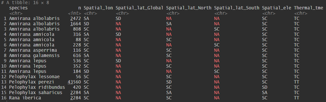
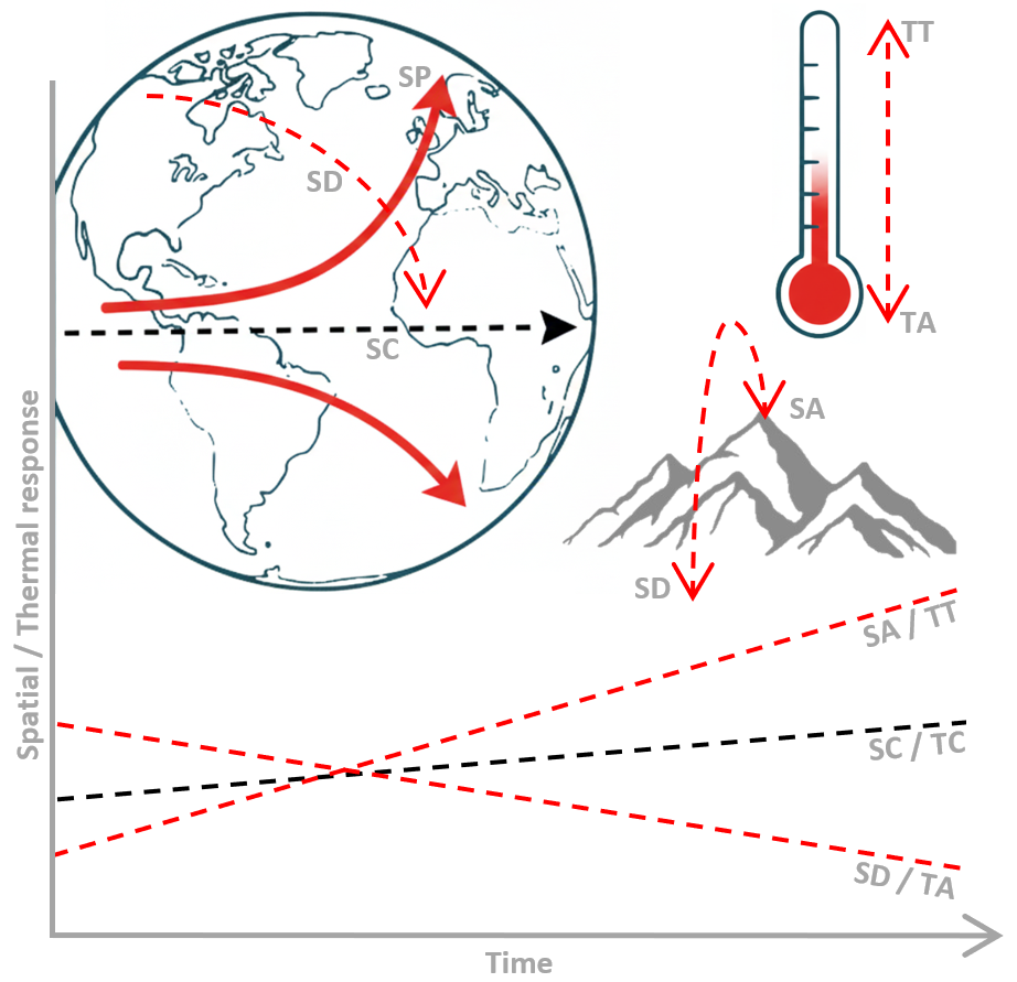
The SppTrend package identifies several Spatial and
Thermal response strategies based on species-specific temporal trends
relative to the overall background trend.
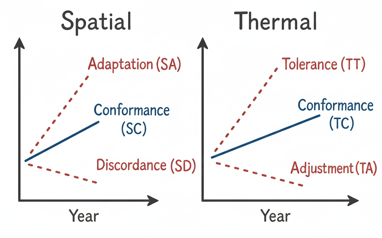
Spatial Responses
Spatial Adaptation (SA): A significant positive temporal trend in the spatial position of species occurrences. In the context of climate change, this pattern is commonly associated with a poleward shift, corresponding to a northward displacement (towards higher latitude values) in the Northern Hemisphere and southward displacement (towards lower latitude values) in the Southern Hemisphere, as species expand into newly suitable areas.
Spatial Discordance (SD): A significant negative temporal trend in the spatial position of species occurrences. In the context of climate change, this pattern is often associated with an equatorward shift and may arise when other ecological and anthropogenic factors influence species distributions independently of, or in opposition to, climate-driven range shifts.
Spatial Conformity (SC): A spatial response pattern in which the species-specific temporal trend does not differ significantly from the overall trend. Species showing spatial conformance share the same bias structure as the complete dataset, preventing the inference of a distinct, species-specific response to climate change at the scale of analysis.
Thermal Responses
Thermal Tolerance (TT): A thermal response pattern characterised by a significant positive temporal trend in the temperature conditions under which species are observed, relative to the overall trend. This pattern suggest an increased likelihood of occurrence under warmer conditions and an apparent capacity to tolerate rising temperatures through physiological, behavioural, and evolutionary mechanisms.
Thermal Adjustment (TA): A thermal response characterised by a significant negative temporal trend in the temperature conditions associated with species occurrences, relative to the overall trend. This indicates and increasing association with cooler temperature conditions over time, potentially reflecting microevolutionary change or phenotypic adjustment.
Thermal Conformity (TC): A thermal response pattern in which species-specific temperature trends do not differ significantly from the overall trend. Species showing thermal conformance share the same background thermal signal as the complete dataset, preventing the formulation of specific hypotheses regarding climate-driven thermal responses.
In essence, while SA and SD describe the ‘what’ (change in presence) and SP/SE a potential ‘how’ (direction of geographic shift along the latitudinal gradient), these spatial responses should be considered together with the thermal responses (TT, TA) to understand if both point towards a consistent overall direction of a species’ response to environmental change.
SppTrend provides a useful methodological framework for
investigating how environmental change affects biodiversity through the
analysis of temporal trends in species occurrence data. However, results
should be interpreted with caution, as opportunistic occurrence data are
inherently subject to multiple sources of bias, including uneven
sampling effort and variation in observer expertise. Although the
overall trend offers a valuable community-level reference, it represents
an average signal across all species and may obscure contrasting
species-specific responses to drivers such as climate warming.
Consequently, emphasis should be placed on species –level trends and
their classification into ecological response strategies, which together
provide a more nuanced and informative understanding of biodiversity
responses to environmental change.
For more detailed information and examples, please refer to the package documentation within R:
help(package = SppTrend)The data used in the example are also available in:
inst/extdata/example_ranidae.csv
path <- system.file("extdata", "example_ranidae.csv", package = "SppTrend")
ranidae <- read_csv(path)This package is based on the methodology described in:
Lobo, Mingarro, Godefroid & García-Roselló (2023) Taking advantage of opportunistically collected historical occurrence data to detect responses to climate change: The case of temperature and Iberian dung beetles. Ecology and evolution, 13(12) e10674. https://doi.org/10.1002/ece3.10674
For any questions or issues, please feel free to contact:
Mario Mingarro mario_mingarro@mncn.csic.es
Jorge M. Lobo jorge.lobo@mncn.csic.es
Emilio García-Roselló egrosello@esei.uvigo.es
These binaries (installable software) and packages are in development.
They may not be fully stable and should be used with caution. We make no claims about them.
Health stats visible at Monitor.