The hardware and bandwidth for this mirror is donated by dogado GmbH, the Webhosting and Full Service-Cloud Provider. Check out our Wordpress Tutorial.
If you wish to report a bug, or if you are interested in having us mirror your free-software or open-source project, please feel free to contact us at mirror[@]dogado.de.
![]()
# vertices
R <- sqrt((5-sqrt(5))/10)     # outer circumradius
r <- sqrt((25-11*sqrt(5))/10) # circumradius of the inner pentagon
X <- R * vapply(0L:4L, function(i) cos(pi/180 * (90+72*i)), numeric(1L))
Y <- R * vapply(0L:4L, function(i) sin(pi/180 * (90+72*i)), numeric(1L))
x <- r * vapply(0L:4L, function(i) cos(pi/180 * (126+72*i)), numeric(1L))
y <- r * vapply(0L:4L, function(i) sin(pi/180 * (126+72*i)), numeric(1L))
vertices <- rbind(
  c(X[1L], Y[1L]),
  c(x[1L], y[1L]),
  c(X[2L], Y[2L]),
  c(x[2L], y[2L]),
  c(X[3L], Y[3L]),
  c(x[3L], y[3L]),
  c(X[4L], Y[4L]),
  c(x[4L], y[4L]),
  c(X[5L], Y[5L]),
  c(x[5L], y[5L])
)
# edge indices (pairs)
edges <- cbind(1L:10L, c(2L:10L, 1L))# constrained Delaunay triangulation
library(RCDT)
del <- delaunay(vertices, edges)# plot
opar <- par(mar = c(0, 0, 0, 0))
plotDelaunay(
del, type = "n", asp = 1, fillcolor = "distinct", lwd_borders = 3,
xlab = NA, ylab = NA, axes = FALSE
)
par(opar)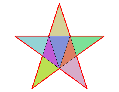
# area
delaunayArea(del)
## [1] 0.3102707
sqrt(650 - 290*sqrt(5)) / 4 # exact value
## [1] 0.3102707I found its vertices with the Julia library Luxor.
vertices <- rbind(
  c(2.121320343559643, 2.1213203435596424),
  c(0.5740251485476348, 1.38581929876693),
  c(0.0, 3.0),
  c(-0.5740251485476346, 1.38581929876693),
  c(-2.1213203435596424, 2.121320343559643),
  c(-1.38581929876693, 0.5740251485476349),
  c(-3.0, 0.0),
  c(-1.3858192987669302, -0.5740251485476345),
  c(-2.121320343559643, -2.1213203435596424),
  c(-0.5740251485476355, -1.3858192987669298),
  c(0.0, -3.0),
  c(0.574025148547635, -1.38581929876693),
  c(2.121320343559642, -2.121320343559643),
  c(1.3858192987669298, -0.5740251485476355),
  c(3.0, 0.0),
  c(1.38581929876693, 0.5740251485476349)
)
# edge indices
edges <- cbind(1L:16L, c(2L:16L, 1L))library(RCDT)
del <- delaunay(vertices, edges)opar <- par(mar = c(0, 0, 0, 0))
plotDelaunay(
del, type = "n", asp = 1, fillcolor = "distinct",
col_borders = "navy", lty_edges = 2, lwd_borders = 3, lwd_edges = 2,
xlab = NA, ylab = NA, axes = FALSE
)
par(opar)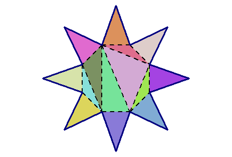
n <- 100L # outer number of sides
angles1 <- seq(0, 2*pi, length.out = n + 1L)[-1L]
outer_points <- cbind(cos(angles1), sin(angles1))
m <- 10L  # inner number of sides
angles2 <- seq(0, 2*pi, length.out = m + 1L)[-1L]
inner_points <- 0.5 * cbind(cos(angles2), sin(angles2))
points <- rbind(outer_points, inner_points)
# constraint edges
indices <- 1L:n
edges_outer <- cbind(
  indices, c(indices[-1L], indices[1L])
)
indices <- n + 1L:m
edges_inner <- cbind(
  indices, c(indices[-1L], indices[1L])
)
edges <- rbind(edges_outer, edges_inner)
# constrained Delaunay triangulation
del <- delaunay(points, edges)
# plot
opar <- par(mar = c(0, 0, 0, 0))
plotDelaunay(
del, type = "n", asp = 1, lwd_borders = 3, col_borders = "black",
fillcolor = "random", col_edges = "yellow",
axes = FALSE, xlab = NA, ylab = NA
)
par(opar)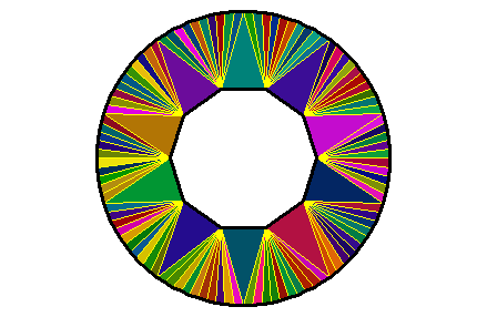
One can also enter a vector of colors in the fillcolor
argument. First, see the number of triangles:
del[["mesh"]]
##  mesh3d object with 110 vertices, 110 triangles.
There are 110 triangles. Let’s make a cyclic vector of 110 colors:
colors <- viridisLite::viridis(55)
colors <- c(colors, rev(colors))
And let’s plot now:
opar <- par(mar = c(0, 0, 0, 0))
plotDelaunay(
  del, type = "n", asp = 1, lwd_borders = 3, col_borders = "black",
  fillcolor = colors, col_edges = "black", lwd_edges = 1.5,
  axes = FALSE, xlab = NA, ylab = NA
)
par(opar)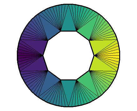
The colors are assigned to the triangles in the order they are given, but only after the triangles have been circularly ordered.
I found this curve here.
t_ <- seq(-pi, pi, length.out = 193L)[-1L]
r_ <- 0.1 + 5*sqrt(cos(6*t_)^2 + 0.7^2)
xy <- cbind(r_*cos(t_), r_*sin(t_))
edges1 <- cbind(1L:192L, c(2L:192L, 1L))
inner <- which(r_ == min(r_))
edges2 <- cbind(inner, c(tail(inner, -1L), inner[1L]))
del <- delaunay(xy, edges = rbind(edges1, edges2))
opar <- par(mar = c(0, 0, 0, 0))
plotDelaunay(
del, type = "n", col_borders = "black", lwd_borders = 2,
fillcolor = "random", col_edges = "white",
axes = FALSE, xlab = NA, ylab = NA, asp = 1
)
polygon(xy[inner, ], col = "#ffff99")
par(opar)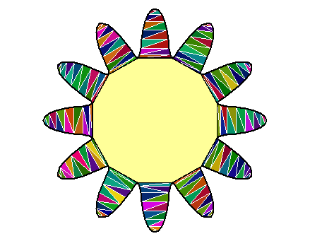
The ‘RCDT’ package as a whole is distributed under GPL-3 (GNU GENERAL PUBLIC LICENSE version 3).
It uses the C++ library CDT which is permissively licensed under MPL-2.0. A copy of the ‘CDT’ license is provided in the file LICENSE.note, and the source code of this library can be found in the src folder.
These binaries (installable software) and packages are in development.
They may not be fully stable and should be used with caution. We make no claims about them.
Health stats visible at Monitor.