The hardware and bandwidth for this mirror is donated by dogado GmbH, the Webhosting and Full Service-Cloud Provider. Check out our Wordpress Tutorial.
If you wish to report a bug, or if you are interested in having us mirror your free-software or open-source project, please feel free to contact us at mirror[@]dogado.de.
![]()
![]()
The goal of {KMunicate} is to produce Kaplan–Meier plots in the style recommended following the KMunicate study (TP Morris et al. Proposals on Kaplan–Meier plots in medical research and a survey of stakeholder views: KMunicate. BMJ Open, 2019, 9:e030215).
You can install {KMunicate} from CRAN by typing the following in your R console:
install.packages("KMunicate")Alternatively, you can install the dev version of {KMunicate} from GitHub with:
# install.packages("devtools")
devtools::install_github("ellessenne/KMunicate-package")library(survival)
library(KMunicate)The {KMunicate} package comes with a couple of bundled dataset,
cancer and brcancer. The main function is
named KMunicate:
KM <- survfit(Surv(rectime, censrec) ~ hormon, data = brcancer)
time_scale <- seq(0, max(brcancer$rectime), by = 365)
KMunicate(fit = KM, time_scale = time_scale)
KM <- survfit(Surv(studytime, died) ~ drug, data = cancer2)
time_scale <- seq(0, max(cancer2$studytime), by = 7)
KMunicate(fit = KM, time_scale = time_scale)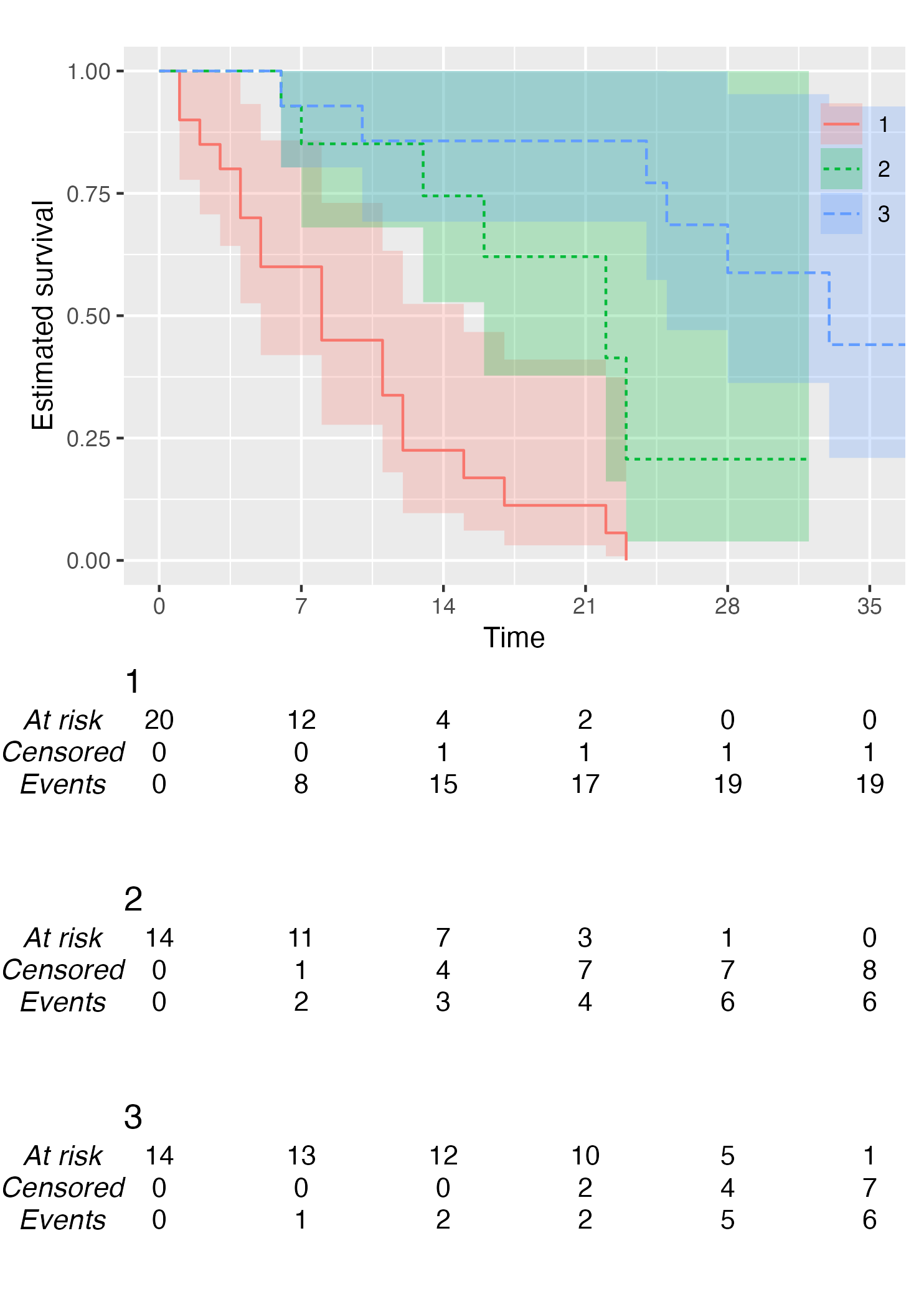
You also might wonder, does this work with a single arm? Yes, yes it does:
KM <- survfit(Surv(studytime, died) ~ 1, data = cancer2)
time_scale <- seq(0, max(cancer2$studytime), by = 7)
KMunicate(fit = KM, time_scale = time_scale)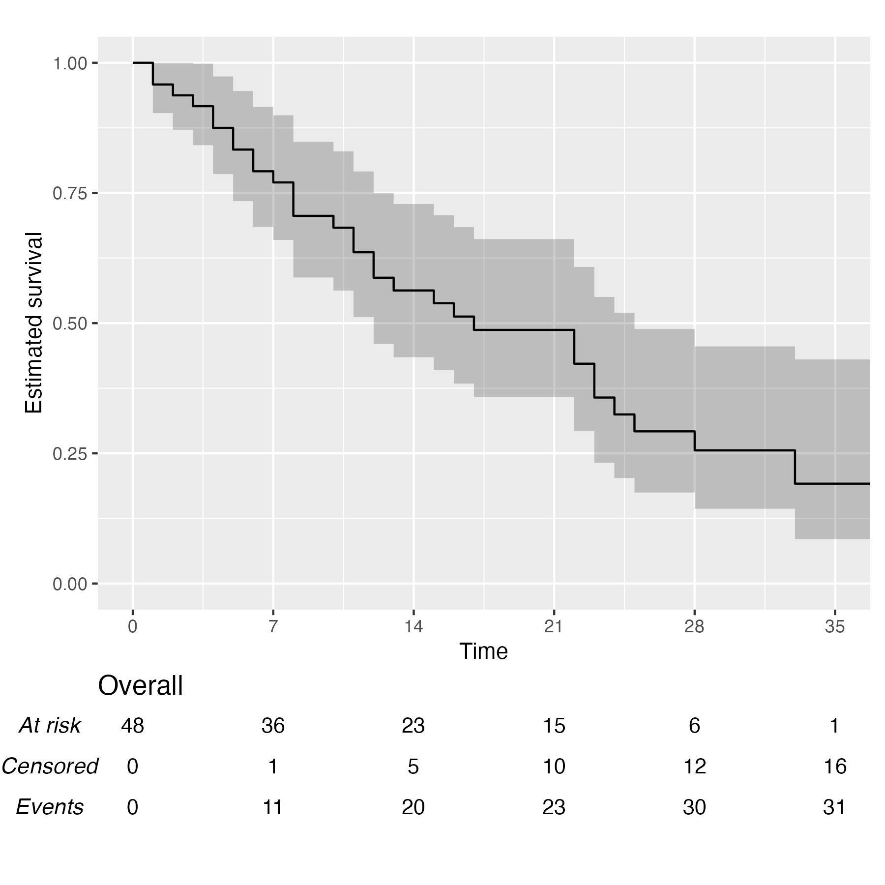
Finally, you can also plot 1 - survival by using the argument
.reverse = TRUE:
KM <- survfit(Surv(rectime, censrec) ~ hormon, data = brcancer)
time_scale <- seq(0, max(brcancer$rectime), by = 365)
KMunicate(fit = KM, time_scale = time_scale, .reverse = TRUE)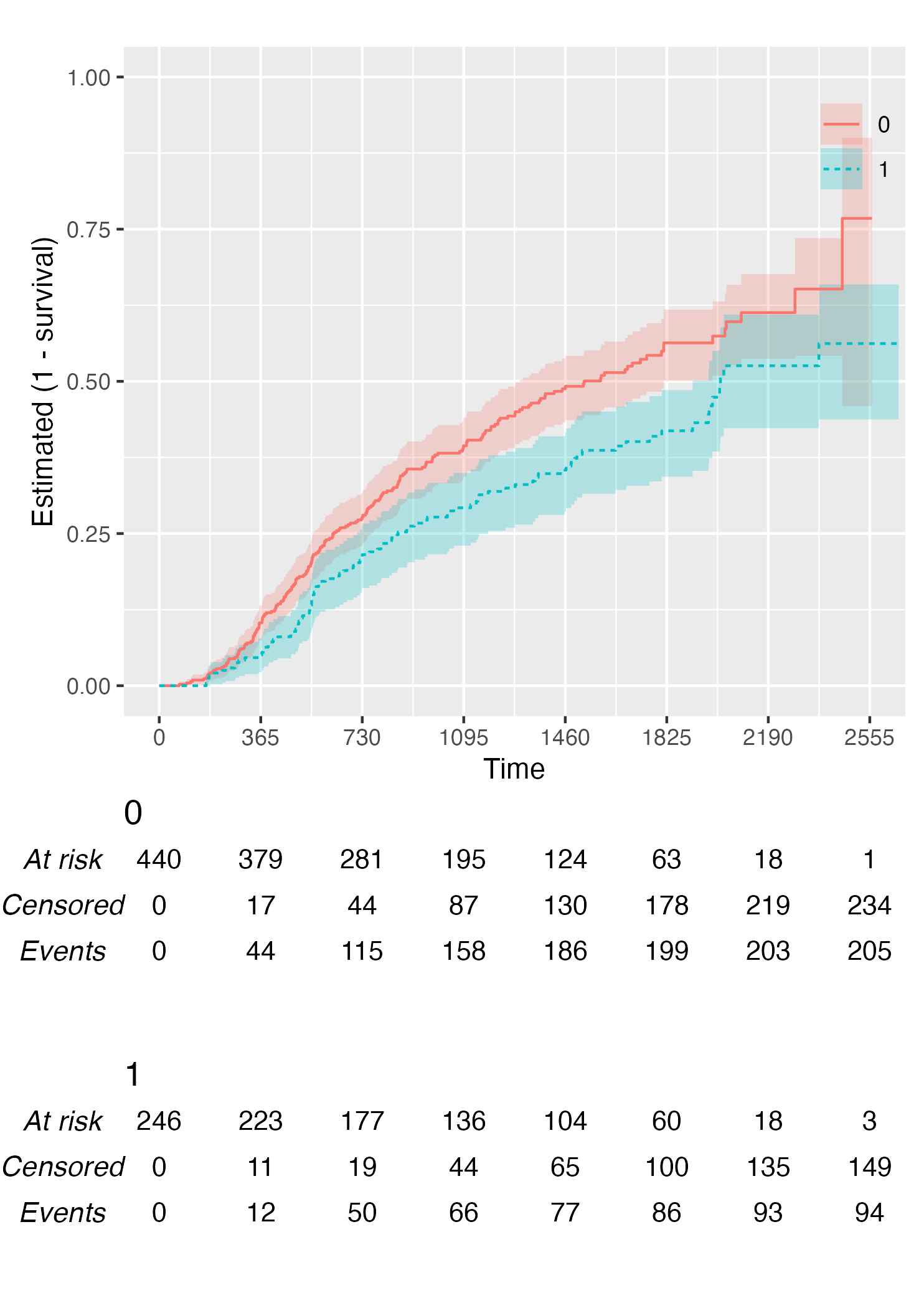
By default, KMunicate() will build a risk table conform
to the KMunicate style, e.g., with cumulative number of events and
censored (the column-wise sum is equal to the total number of
individuals at risk per arm):
KM <- survfit(Surv(rectime, censrec) ~ hormon, data = brcancer)
time_scale <- seq(0, max(brcancer$rectime), by = 365)
KMunicate(fit = KM, time_scale = time_scale)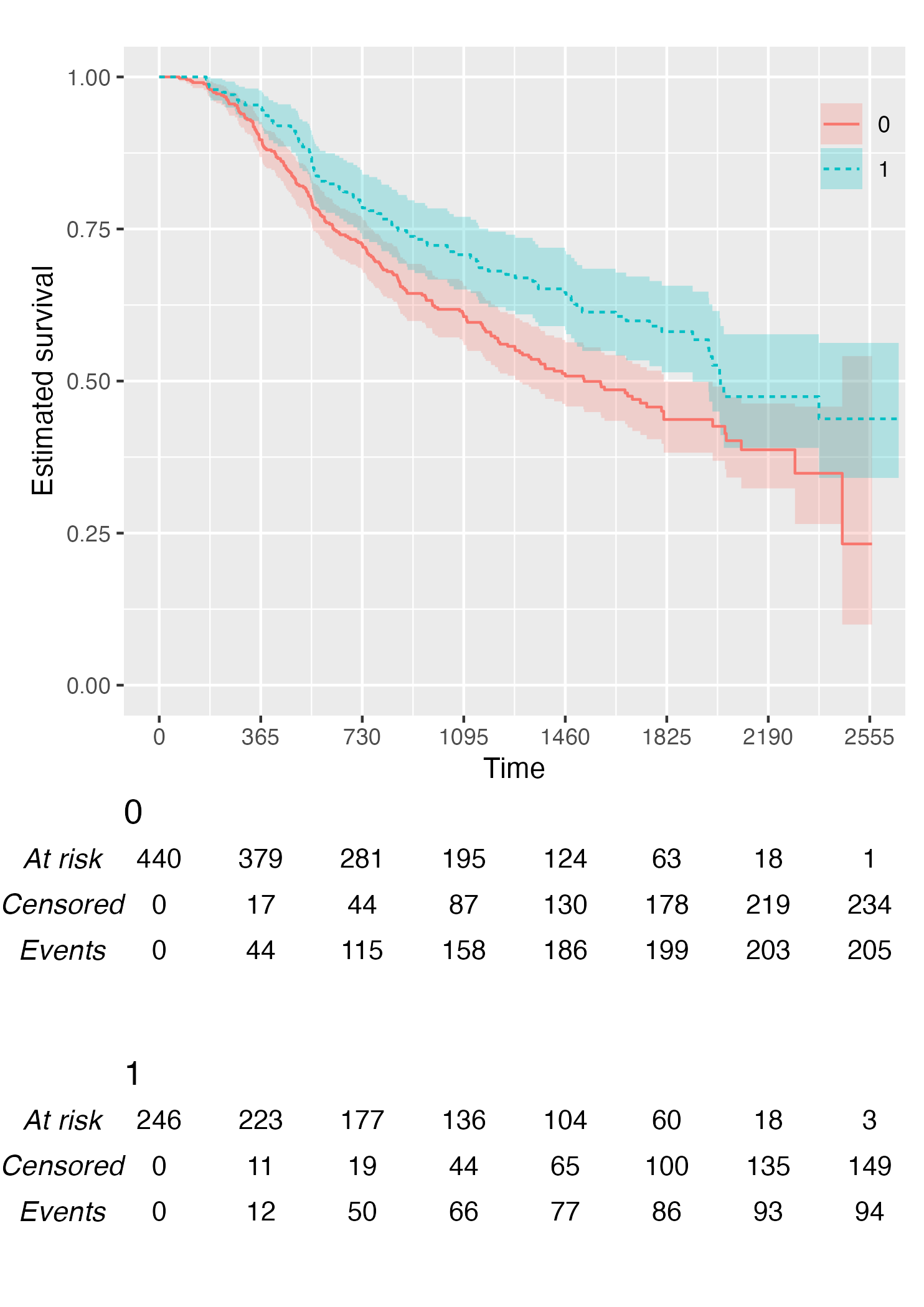
Alternatively, it is possible to customise the risk table via the
.risk_table argument. For instance, if one wants to have
interval-wise number of events and censored, just pass the
survfit value to the .risk_table argument:
KMunicate(fit = KM, time_scale = time_scale, .risk_table = "survfit")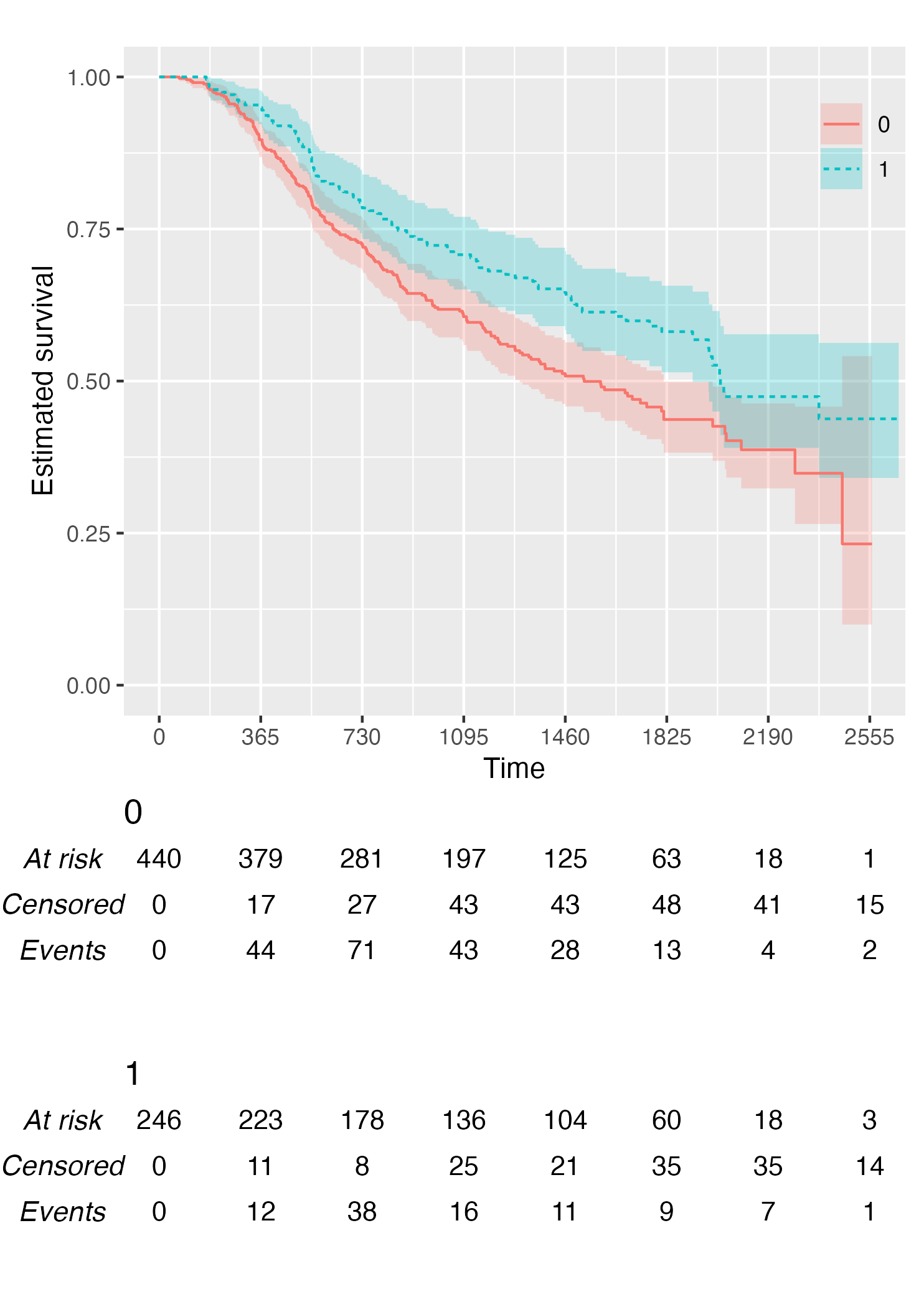
This is the default output of the summary.survfit()
function.
Finally, it is also possible to fully omit the risk table by setting
.risk_table = NULL:
KMunicate(fit = KM, time_scale = time_scale, .risk_table = NULL)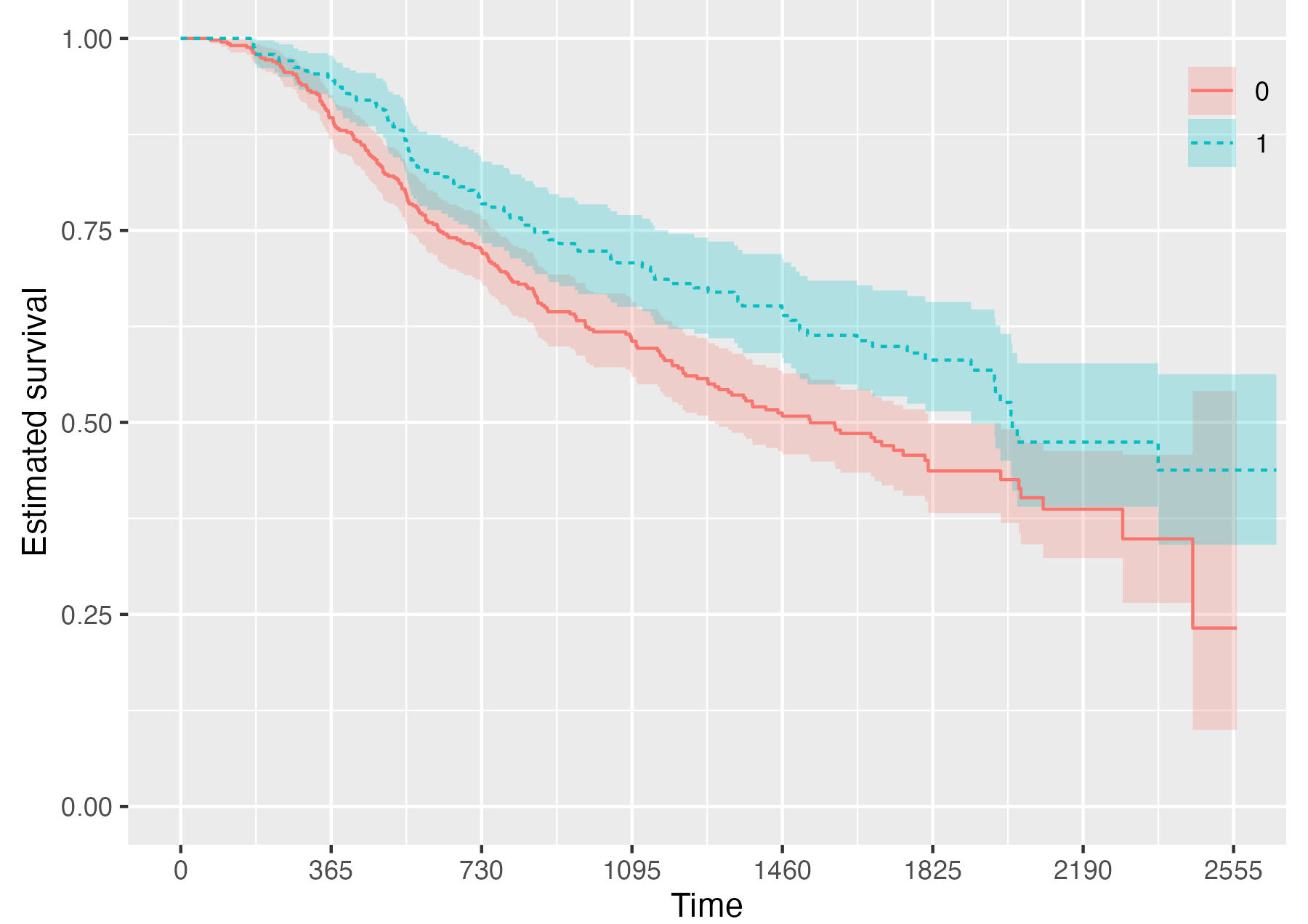
Assuming you have set up your computer to use custom fonts with
ggplot2, customising your KMunicate-style plot is trivial.
All you have to do is pass the font name as the .ff
argument:
KM <- survfit(Surv(studytime, died) ~ 1, data = cancer2)
time_scale <- seq(0, max(cancer2$studytime), by = 7)
KMunicate(fit = KM, time_scale = time_scale, .ff = "Times New Roman")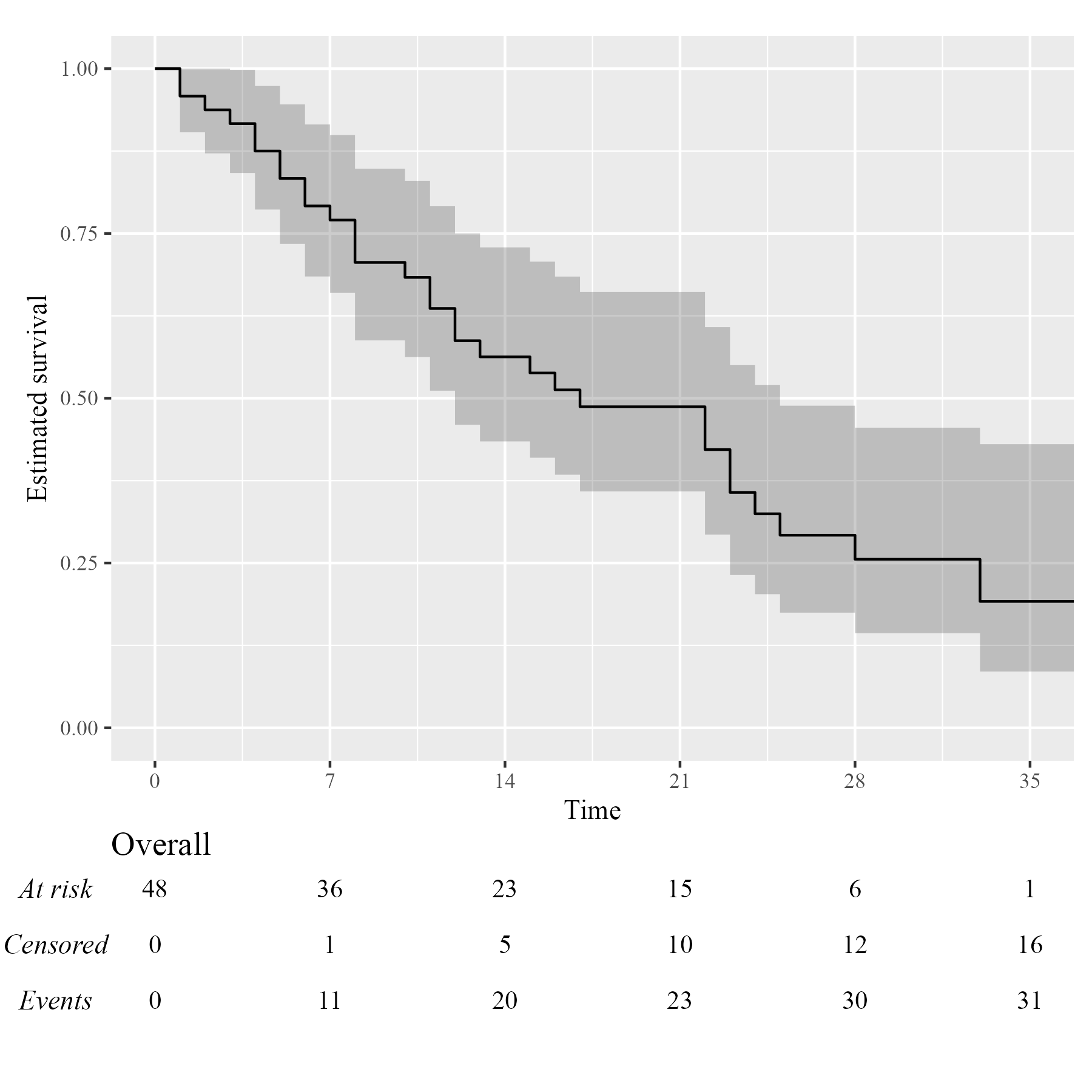
Several options to further customise each plot are provided, see e.g. the introductory vignette for more details.
These binaries (installable software) and packages are in development.
They may not be fully stable and should be used with caution. We make no claims about them.
Health stats visible at Monitor.