The hardware and bandwidth for this mirror is donated by dogado GmbH, the Webhosting and Full Service-Cloud Provider. Check out our Wordpress Tutorial.
If you wish to report a bug, or if you are interested in having us mirror your free-software or open-source project, please feel free to contact us at mirror[@]dogado.de.
![]()
Gmisc collects utilities for the graphics and tables
that recur in medical research papers — built so they compose with the
native R pipe (|>):
getDescriptionStatsBy() + htmlTable() for
publication-ready, copy-paste descriptive tables.flowchart() |> spread() |> move() |> connect()
pipeline for CONSORT-style diagrams, including phaseLabel()
headings.Transition
class for visualising how observations move between categories over
time.getSvdMostInfluential() for picking influential
variables.grid package.# From CRAN
install.packages("Gmisc")
# Development version from GitHub
# install.packages("remotes")
remotes::install_github("gforge/Gmisc")Build a flowchart as a named list of boxes, position the columns with
spread()/move(), then add the connectors.
Parallel arms are just lists, and phaseLabel() drops a
CONSORT phase heading (“Allocation”, “Follow-up”, …) between the arms —
centred, slightly overlapping, and drawn on top.
library(Gmisc)
library(grid)

main_gp <- gpar(fill = "white", col = "black", lwd = 1)
head_gp <- gpar(fill = "#c8daf7", col = "#2f5f9f", lwd = 1)
con_gp  <- gpar(col = "#4f86c6", fill = "#4f86c6", lwd = 1.8)
sw      <- unit(70, "mm")

flowchart(
  rando = boxGrob("Randomised\nN = 100", box_gp = main_gp),
  groups = list(
    boxGrob("Allocated to intervention\nn = 50", width = sw, box_gp = main_gp),
    boxGrob("Allocated to control\nn = 50", width = sw, box_gp = main_gp)
  ),
  followup = list(
    boxGrob("Lost to follow-up\nn = 1", width = sw, box_gp = main_gp),
    boxGrob("Lost to follow-up\nn = 2", width = sw, box_gp = main_gp)
  ),
  analysis = list(
    boxGrob("Analysed\nn = 49", width = sw, box_gp = main_gp),
    boxGrob("Analysed\nn = 48", width = sw, box_gp = main_gp)
  )
) |>
  spread(axis = "y", margin = unit(0.04, "npc")) |>
  move(subelement = list(c("groups", 1), c("followup", 1), c("analysis", 1)), x = 0.27) |>
  move(subelement = list(c("groups", 2), c("followup", 2), c("analysis", 2)), x = 0.73) |>
  phaseLabel("groups",   "Allocation", box_gp = head_gp) |>
  phaseLabel("followup", "Follow-up",  box_gp = head_gp) |>
  phaseLabel("analysis", "Analysis",   box_gp = head_gp) |>
  connect("rando",    "groups",   type = "N", lty_gp = con_gp, arrow_size = 3, smooth = TRUE) |>
  connect("groups",   "followup", type = "v", lty_gp = con_gp, arrow_size = 3) |>
  connect("followup", "analysis", type = "v", lty_gp = con_gp, arrow_size = 3)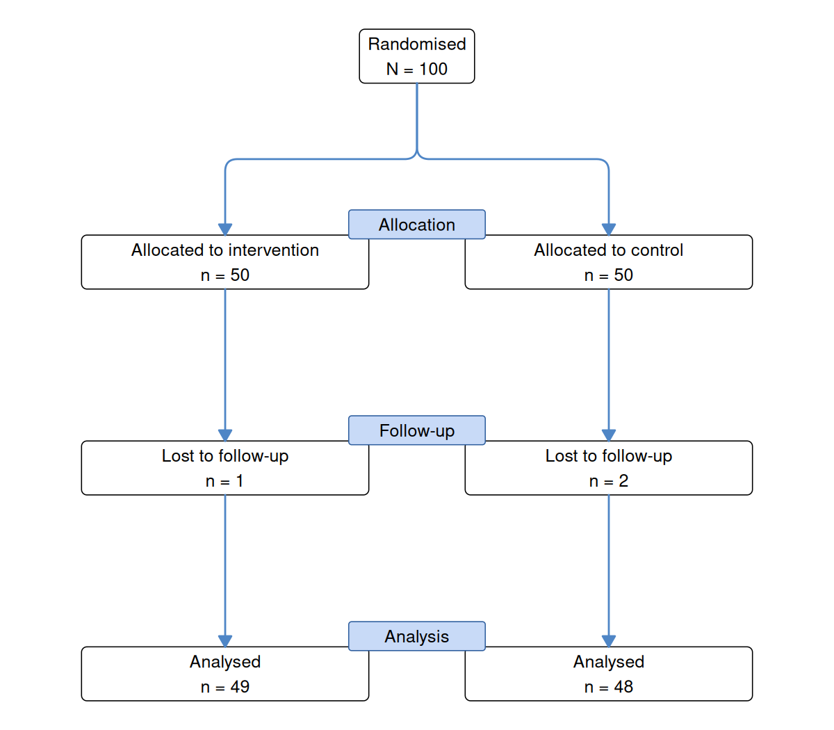
See vignette("Grid-based_flowcharts", package = "Gmisc")
for the full API.
getDescriptionStatsBy() summarises variables split by a
grouping column. It is often used with mergeDesc() to group
related variables into sections, and pipes straight into
htmlTable() for a publication-ready table.
library(dplyr)
library(Gmisc)
# A custom wrapper to keep statistics and formatting consistent
# (e.g., same digits, p-values, and header count)
get_stats <- function(data, ...) {
res <- data |>
getDescriptionStatsBy(...,
by = am,
statistics = TRUE,
digits = 1,
header_count = TRUE)
if (is.list(res)) {
return(do.call(rbind, res))
}
return(res)
}
mtcars_prep <- mtcars |>
mutate(am = factor(am, labels = c("Automatic", "Manual")),
gear = factor(gear),
cyl = factor(cyl)) |>
set_column_labels(mpg = "Gas",
wt = "Weight",
hp = "Horsepower",
cyl = "Cylinders",
gear = "Gears") |>
set_column_units(mpg = "Miles/gallon",
wt = "10<sup>3</sup> lbs",
hp = "hp")
# Group variables and merge them into a single table
mergeDesc(
"Main" = mtcars_prep |> get_stats(mpg, wt),
"Engine" = mtcars_prep |> get_stats(hp, cyl),
"Transmission" = mtcars_prep |> get_stats(gear)
) |>
htmlTable(caption = "Baseline characteristics by transmission",
tfoot = "† Statistics: Mean (SD) for continuous; n (%) for categorical")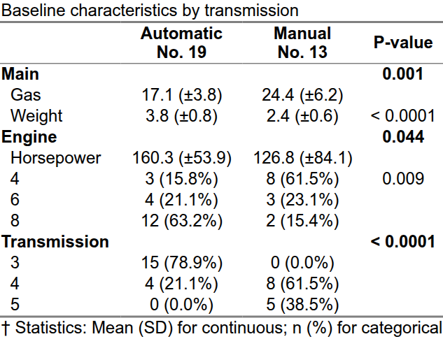
See vignette("Descriptives", package = "Gmisc") for the
many formatting options.
The Transition class shows how observations move between
classes over time; a third dimension can be encoded as a colour split
within each box.
set.seed(1)
n <- 100
sex    <- sample(c("Male", "Female"), n, replace = TRUE)
before <- sample(1:3, n, replace = TRUE)
# Most cases improve one class, some stay, a few worsen
after  <- pmin(pmax(before - sample(c(-1, 0, 1), n, replace = TRUE, prob = c(.15, .35, .5)), 1), 3)

lbl <- c("A", "B", "C")
tbl <- table(factor(before, 1:3, lbl), factor(after, 1:3, lbl), sex)

transitions <- getRefClass("Transition")$new(tbl, label = c("Before surgery", "1 year after"))
transitions$title   <- "Charnley class before vs. after surgery"
transitions$clr_bar <- "bottom"
transitions$render()![]()
See vignette("Transition-class", package = "Gmisc") for
customisation.
browseVignettes("Gmisc")These binaries (installable software) and packages are in development.
They may not be fully stable and should be used with caution. We make no claims about them.
Health stats visible at Monitor.