The hardware and bandwidth for this mirror is donated by dogado GmbH, the Webhosting and Full Service-Cloud Provider. Check out our Wordpress Tutorial.
If you wish to report a bug, or if you are interested in having us mirror your free-software or open-source project, please feel free to contact us at mirror[@]dogado.de.
![]()
The goal of EcoCleanR is to provides functions to integrate biodiversity data from multiple aggregates and offers a step-by-step framework for data cleaning, outlier detection, and the generation of species biogeographic ranges. It also supports the extraction of relevant environmental information to assist in ecological and conservation analyses.
Key features:
install.package("EcoCleanR")#cran versionInstall the development version of EcoCleanR from GitHub:
How to install package from github or through zip file downloaded
from github:
Install devtools and remotes packages and load
them.
#install.packages(“devtools”)
#install.packages(“remotes”)
#library(devtools)
#library(remotes)
Install EcoCleanR package from [github] development version
#remotes::install_github(“sonipri/EcoCleanR”)
or install EcoCleanR package from downloaded zip
file.
  #devtools::install_local("EcoCleanR.zip",
  dependencies = TRUE)
unzip the zip file EcoCleanR and set it as working
directory.
#setwd(…path)
Optional: Only for testing purposes.
#devtools::check()
see data merging steps vignette:
[data_merging]
see data cleaning steps on merged dataset at vignette:
[data_cleaning]
Recommanded :see the Step-by-Step Workflow for complete process — from data downloading, processing, merging, cleaning, and visualization at vignettes/article/stepbystep.rmd.
This is a basic example to demonstrate data processing, merging and cleanings steps for a species name “Mexacanthina lugubris”
library(EcoCleanR)
## basic example code
# After execution of step 1 and 2.1, output file called "ecodata"
# This dataset contains ~1100 occurrence records for the species Mexacanthina lugubris. It was compiled by merging data from multiple online repositories — GBIF, OBIS, iDigBio and local file (InvertEbase) — consider as step 1 (Vignette: data_merging). Duplicate records were removed to retain only unique occurrences (2.1) using function "ec_rm_duplicate".
# The algorithm for these steps can be found on article folder - documentation
head(ecodata)
#>   X basisOfRecord occurrenceStatus institutionCode
#> 1 1        modern          PRESENT     iNaturalist
#> 2 2        modern          PRESENT             CAS
#> 3 3        modern          PRESENT     iNaturalist
#> 4 4        modern          PRESENT             CAS
#> 5 5        modern          PRESENT     iNaturalist
#> 6 6        modern          PRESENT              LI
#>                         verbatimEventDate
#> 1 Tue Nov 02 2021 12:32:42 GMT-0700 (PDT)
#> 2                                2-Jan-75
#> 3 Sat Nov 13 2021 14:00:19 GMT-0800 (PST)
#> 4                                1-Jan-75
#> 5                  2021/03/19 3:34 PM CDT
#> 6                                    <NA>
#>                                scientificName individualCount organismQuantity
#> 1 Mexacanthina lugubris (G.B.Sowerby I, 1822)              NA               NA
#> 2 Mexacanthina lugubris (G.B.Sowerby I, 1822)              NA               NA
#> 3 Mexacanthina lugubris (G.B.Sowerby I, 1822)              NA               NA
#> 4 Mexacanthina lugubris (G.B.Sowerby I, 1822)              NA               NA
#> 5 Mexacanthina lugubris (G.B.Sowerby I, 1822)              NA               NA
#> 6       Acanthina tyrianthina S.S.Berry, 1957              NA               NA
#>   abundance decimalLatitude decimalLongitude coordinateUncertaintyInMeters
#> 1        NA        33.51358        -117.7583                            65
#> 2        NA              NA               NA                            NA
#> 3        NA        32.81539        -117.2741                            83
#> 4        NA              NA               NA                            NA
#> 5        NA        32.67190        -117.2455                            12
#> 6        NA              NA               NA                            NA
#>                                                                                   locality
#> 1                                                                                     <NA>
#> 2    Pacific Ocean, Guadalupe Island [Isla Guadalupe], Old Sealer's Cove, intertidal pools
#> 3                                                                                     <NA>
#> 4 Pacific Ocean, Guadalupe Island [Isla Guadalupe], Old Sealer's Cove, bare rocks, exposed
#> 5                                                                                     <NA>
#> 6                                                     La Bujadera, Baja California, Mexico
#>                            verbatimLocality municipality county stateProvince
#> 1 North Pacific Ocean, Laguna Beach, CA, US           NA   <NA>    California
#> 2                                      <NA>           NA   <NA>          <NA>
#> 3               North Pacific Ocean, CA, US           NA   <NA>    California
#> 4                                      <NA>           NA   <NA>          <NA>
#> 5                        San Diego, CA, USA           NA   <NA>    California
#> 6                                      <NA>           NA   <NA>          <NA>
#>                    country cleaned_catalog
#> 1 United States of America       100088422
#> 2                   Mexico            1001
#> 3 United States of America       101101719
#> 4                   Mexico            1016
#> 5 United States of America       101984642
#> 6 United States of America       102083202

# visualizing the raw data
ec_geographic_map(ecodata,
  latitude = "decimalLatitude",
  longitude = "decimalLongitude"
)
#> Warning: Removed 358 rows containing missing values or values outside the scale range
#> (`geom_point()`).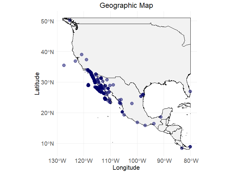
# lets execute cleaning steps
# step 2.2 - check taxon error for species name - "Mexacanthina lugubris"
comparison <- ec_worms_synonym(
  "Mexacanthina lugubris",
  ecodata,
  scientificName = "scientificName"
)
#> ══  1 queries  ═══════════════
#>
#> Retrieving data for taxon 'Mexacanthina lugubris'
#> ✔  Found:  Mexacanthina lugubris
#> ══  Results  ═════════════════
#>
#> • Total: 1
#> • Found: 1
#> • Not Found: 0
# step 2.3 - check records with locality but no coordinate assignments
ecodata$flag_with_locality <- ec_flag_with_locality(
  ecodata,
  uncertainty = "coordinateUncertaintyInMeters",
  locality = "locality",
  verbatimLocality = "verbatimLocality"
)
# upload back the corrected file with csv upload - name it as ecodata_corrected
head(ecodata_corrected)
#>   cleaned_catalog corrected_latitude corrected_longitude corrected_uncertainty
#> 1            1001           29.03741           -118.3182                 19180
#> 2            1016           29.03741           -118.3182                 19180
#> 3       102443960           32.72160           -117.2112                 23582
#> 4       104087711           32.66767           -117.2452                  1771
#> 5       104911613           32.72160           -117.2112                 23284
#> 6       105885508           32.83330           -117.2667                  2962
ecodata <- ec_merge_corrected_coordinates(
  ecodata_corrected,
  ecodata,
  latitude = "decimalLatitude",
  longitude = "decimalLongitude",
  uncertainty_col = "coordinateUncertaintyInMeters"
)

ecodata <- ec_filter_by_uncertainty(
  ecodata,
  uncertainty_col = "coordinateUncertaintyInMeters",
  percentile = 0.95,
  ask = TRUE,
  latitude = "decimalLatitude",
  longitude = "decimalLongitude"
)
#> Suggested threshold at 95th percentile: 24015.45
#> Do you want to apply this threshold? (y/n):
#> No filtering applied.

# step 2.4 - check records with bad precision <2 as well as rounding issue
ecodata$flag_precision <- ec_flag_precision(
  ecodata,
  latitude = "decimalLatitude",
  longitude = "decimalLongitude"
)
# step 2.5 - check records with wrong assignment of ocean/sea and inland with certain buffer range - not executing on run
if (FALSE) {
  ecodata$flag_non_region <- ec_flag_non_region(
    "east",
    "pacific",
    buffer = 25000,
    ecodata,
    latitude = "decimalLatitude",
    longitude = "decimalLongitude"
  )
}
# step 2.6 - extract the environmental variables, here we are using a data table which has unique combination of coordinates - we call it ecodata_x - not executing on run
if (FALSE) {
  env_layers <- c("BO_sstmean", "BO_sstmax", "BO_sstmin")
  ecodata_x <- ec_extract_env_layers(ecodata_x,
    env_layers = env_layers,
    latitude = "decimalLatitude",
    longitude = "decimalLongitude"
  )
}
# step 2.7 - impute the environmental variables for those coordinates with no assignment on online data sources.
if (FALSE) {
  ecodata_x <- ec_impute_env_values(ecodata_x, radius_km, iter)
}
# step 2.8 - calculate outlier probability for each data points.
if (FALSE) {
  ecodata_x$flag_outliers <- ((
    ec_flag_outlier(
      ecodata_x,
      latitude = "decimalLatitude",
      longitude = "decimalLongitude",
      env_layers,
      itr = 100,
      k = 3,
      geo_quantile = 0.99,
      maha_quantile = 0.99
  )))$ouliers
}
# step 3.1 - visualize the map with outlier probability index, bind the ecodata_x with ecodata with updated column flag_outlier
ec_geographic_map_w_flag(
  ecodata_with_outliers,
  flag_column = "outliers",
  latitude = "decimalLatitude",
  longitude = "decimalLongitude"
)
#> Ignoring unknown labels:
#> • colour : "Flag"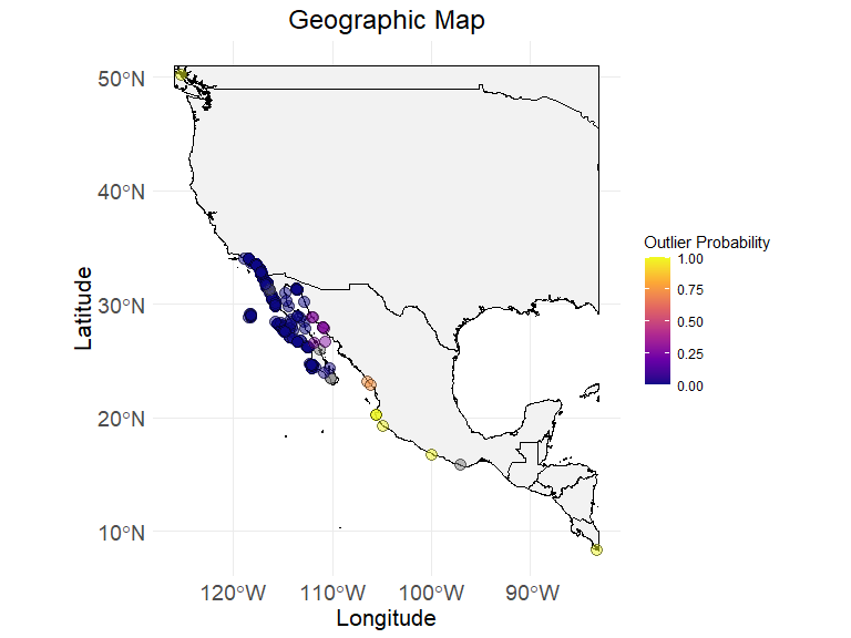
# at this stage we can decide the acceptable outlier probability and after removing higher probable a new datafram called ecodata_cleaned can be source of summary table (next step)
# step 3.2 - Visualize the summary table
env_layers <- c("BO_sstmean", "BO_sstmax", "BO_sstmin")
data("ecodata_cleaned")
ec_geographic_map(ecodata_cleaned)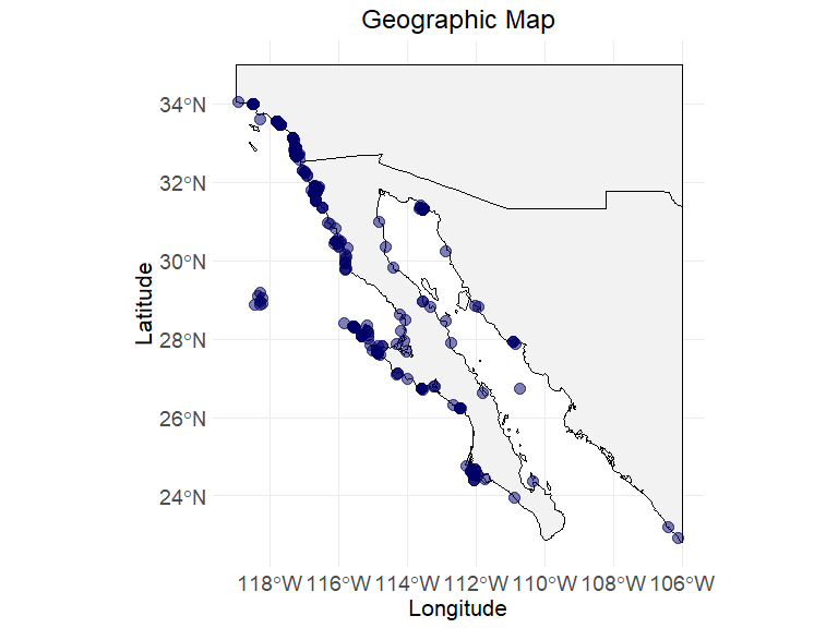
summary_table <- ec_var_summary(
ecodata_cleaned,
latitude = "decimalLatitude",
longitude = "decimalLongitude",
env_layers
)
print(summary_table)
#> variable Max Min Mean
#> 1 decimalLatitude 34.04 22.92 31.73
#> 2 decimalLongitude -106.10 -118.94 -116.58
#> 3 BO_sstmean 29.04 16.15 17.97
#> 4 BO_sstmax 32.68 18.79 22.47
#> 5 BO_sstmin 24.96 11.42 14.41
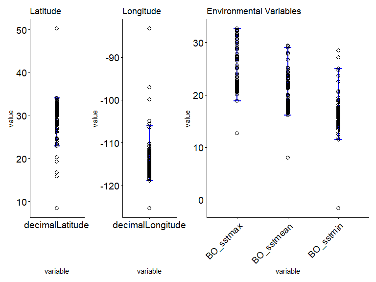
# step 3.3 - Plot to visual the acceptable limit of a species which demonstrate a suitable habitat range:
ec_plot_var_range(
ecodata_with_outliers,
summary_table,
latitude = "decimalLatitude",
longitude = "decimalLongitude",
env_layers
)
Further documents:
*see data merging vignette: [data_merging]
*see data cleaning steps on merged dataset at vignette:
[data_cleaning]
*see the Step-by-Step Workflow vignette for a detailed explanation of
the complete process — from data downloading to merging, cleaning, and
visualization at vignettes/article/stepbystep.rmd.
*see citation guidelines for the downloaded data from gbif, obis, idigbio and InvertEbase [cite_data] at vignettes/article/cite_data.rmd.
These binaries (installable software) and packages are in development.
They may not be fully stable and should be used with caution. We make no claims about them.
Health stats visible at Monitor.